Introduction
This article shows the methodology used to classify EV charging sessions among generic user profiles, using the R package evprof. The goal of this analysis is to define generic user profiles or, in other words, EV connection patterns that could relate a charging sessions to a specific user behaviour. The most relevant variables of the data set are the Connection Start Time and the Connection Hours (duration). Based on these two variables evprof package aims to provide tools to analyze, cluster and model different user profiles with similar flexibility potential to, in a farther stage, exploit their flexibility in specific demand response programs.
The workflow followed to perform in this tutorial is the one below:
- Data exploratory analysis
- Data set visualization
- Statistic analysis
- Pre-processing
- Data division
- Outliers cleaning
- Clustering
- Profiling
- Modelling
- Simulation
- Comparison of simulation with real data
This article applies the methodology proposed to a real EV data set
from a mid-sized Dutch city. However, the aim of package
evprof is to replicate the same methodology to other real
data sets for any other country in the world, like the example data set
of EV charging sessions provided by evprof (see the California
article). If you use this package don’t hesitate to comment your
results with the authors of evprof.
Data exploratory analysis
Data set visualization
This charging sessions data set contains 210711 sessions, from
2015-08-31 to 2020-06-01. The variables in the data set must have the
evprof standard format described in
vignette("sessions-format").
| Session | ConnectionStartDateTime | ConnectionEndDateTime | ChargingStartDateTime | ChargingEndDateTime | Power | Energy | ConnectionHours | ChargingHours | FlexibilityHours | ChargingStation |
|---|---|---|---|---|---|---|---|---|---|---|
| 85851 | 2015-08-31 17:53:00 | 2015-09-02 07:17:00 | 2015-08-31 17:53:00 | 2015-08-31 22:18:00 | 2.231386 | 9.89 | 37.40000 | 4.4322222 | 32.967778 | NLAMSEARNH0007 |
| 86339 | 2015-09-01 15:28:00 | 2015-09-02 12:21:00 | 2015-09-01 15:28:00 | 2015-09-01 16:44:00 | 1.965202 | 2.51 | 20.88333 | 1.2772222 | 19.606111 | NLAMSEARNH0012 |
| 86305 | 2015-09-01 17:41:00 | 2015-09-02 07:06:00 | 2015-09-01 17:41:00 | 2015-09-01 22:14:00 | 2.326762 | 10.59 | 13.41667 | 4.5513889 | 8.865278 | NLAMSEARNH0036 |
| 86329 | 2015-09-01 18:08:00 | 2015-09-02 07:10:00 | 2015-09-01 18:08:00 | 2015-09-01 19:14:00 | 1.737120 | 1.92 | 13.03333 | 1.1052778 | 11.928056 | NLAMSEARNH0019 |
| 86332 | 2015-09-01 18:12:00 | 2015-09-02 08:11:00 | 2015-09-01 18:12:00 | 2015-09-01 21:39:00 | 2.816110 | 9.75 | 13.98333 | 3.4622222 | 10.521111 | NLALLEGO000328 |
| 86336 | 2015-09-01 18:19:00 | 2015-09-02 07:45:00 | 2015-09-01 18:19:00 | 2015-09-02 00:54:00 | 3.052055 | 20.13 | 13.43333 | 6.5955556 | 6.837778 | NLAMSEARNH0033 |
| 86354 | 2015-09-01 18:33:00 | 2015-09-02 07:21:00 | 2015-09-01 18:33:00 | 2015-09-01 20:44:00 | 3.481669 | 7.65 | 12.80000 | 2.1972222 | 10.602778 | NLAMSEARNH0027 |
| 86361 | 2015-09-01 19:22:00 | 2015-09-02 08:38:00 | 2015-09-01 19:22:00 | 2015-09-01 23:59:00 | 2.214286 | 10.23 | 13.26667 | 4.6200000 | 8.646667 | NLALLEGO000283 |
| 86376 | 2015-09-01 19:59:00 | 2015-09-02 07:11:00 | 2015-09-01 19:59:00 | 2015-09-01 21:54:00 | 3.403166 | 6.57 | 11.20000 | 1.9305556 | 9.269444 | NLAMSEARNH0004 |
| 86371 | 2015-09-01 20:00:00 | 2015-09-05 14:49:00 | 2015-09-01 20:00:00 | 2015-09-01 20:44:00 | 2.057527 | 1.53 | 90.81667 | 0.7436111 | 90.073056 | NLAMSEARNH0018 |
The following plot represents with a point every charging session in hour data set, based on the two most relevant features to define a user profile: Connection Start Time and Connection Hours (duration).
plot_points(sessions, size = 0.25)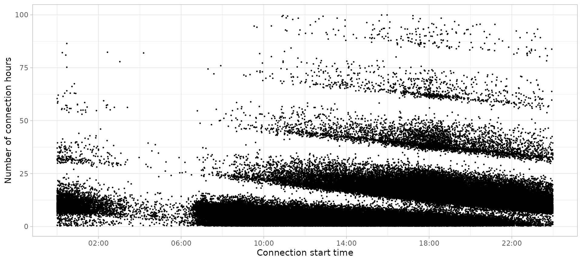
As you can see, the visible “clouds” of points are not plotted in
their natural shape. They are cut because the x axis of the plot goes
from 00:00 to 23:59 of a single day, while the connection patterns start
from 6 AM of one day until the morning of the next day. To solve this
issue, a lot of evprof functions have a start
parameter to set up the hour from which the EV users start their
connections.
plot_points(sessions, start = 6, size = 0.25)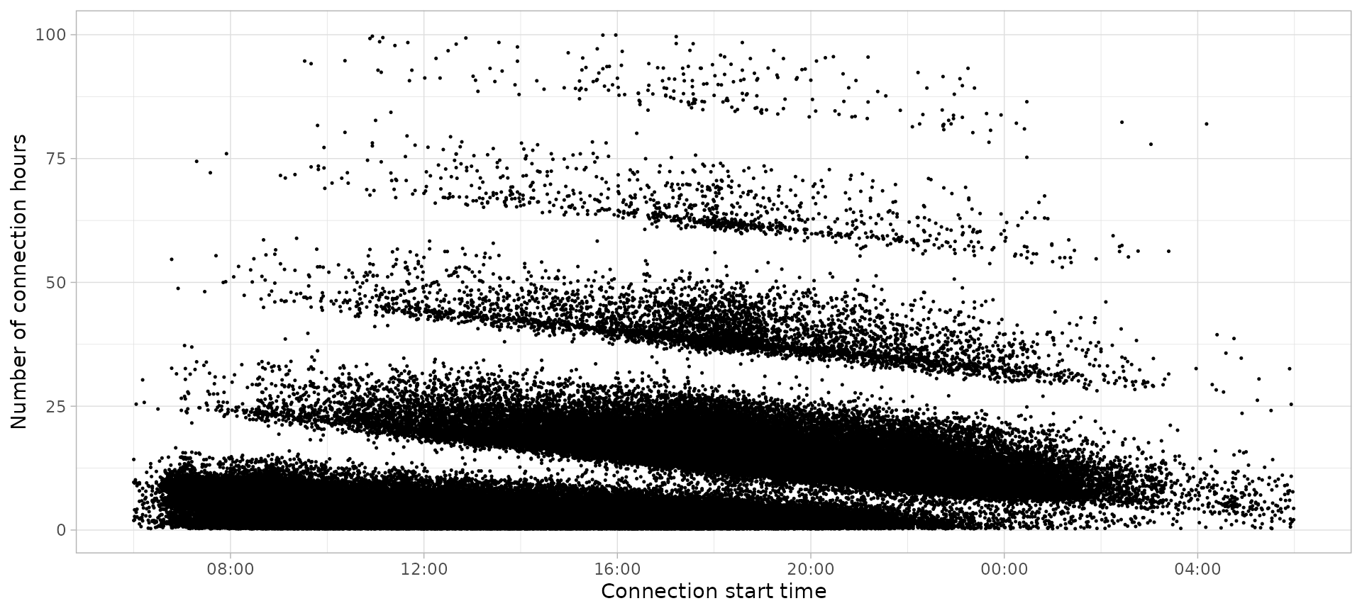
This start parameter can be defined with a global option
since most function have the default value as
start = getOption("evprof.start.hour"). Since this
parameter depends on the use case, we recommend to define it at the
beginning of the analysis:
options(
  evprof.start.hour = 6
)
Statistic analysis
The average values of the most important features in our charging sessions data set are:
summarise_sessions(sessions, mean) %>%
knitr::kable(digits = 2)| Power | Energy | ConnectionHours | ChargingHours | FlexibilityHours |
|---|---|---|---|---|
| 4.27 | 12.41 | 9.62 | 2.84 | 6.78 |
Even though average values don’t give a clear view of the sessions, in general our data set has:
- Low charging power (new EV models can charge up to 22 kW AC), probably most of sessions charge with 3.7 or 7.3 kW rates.
- Low energy demand (most of models have at least 40 kWh of battery), probably due to the energy spent in the travel home-city.
- Long connections, probably during the night.
- Low charging hours due to low energy demand.
- High flexibility due to long connections and low energy demand.
However, the goal of analyzing different user profiles is to find groups of sessions with different features averages. A more depth overview of the data set in this sense can be done with a distribution plot (histogram) of each one of these features:
plot_histogram_grid(sessions)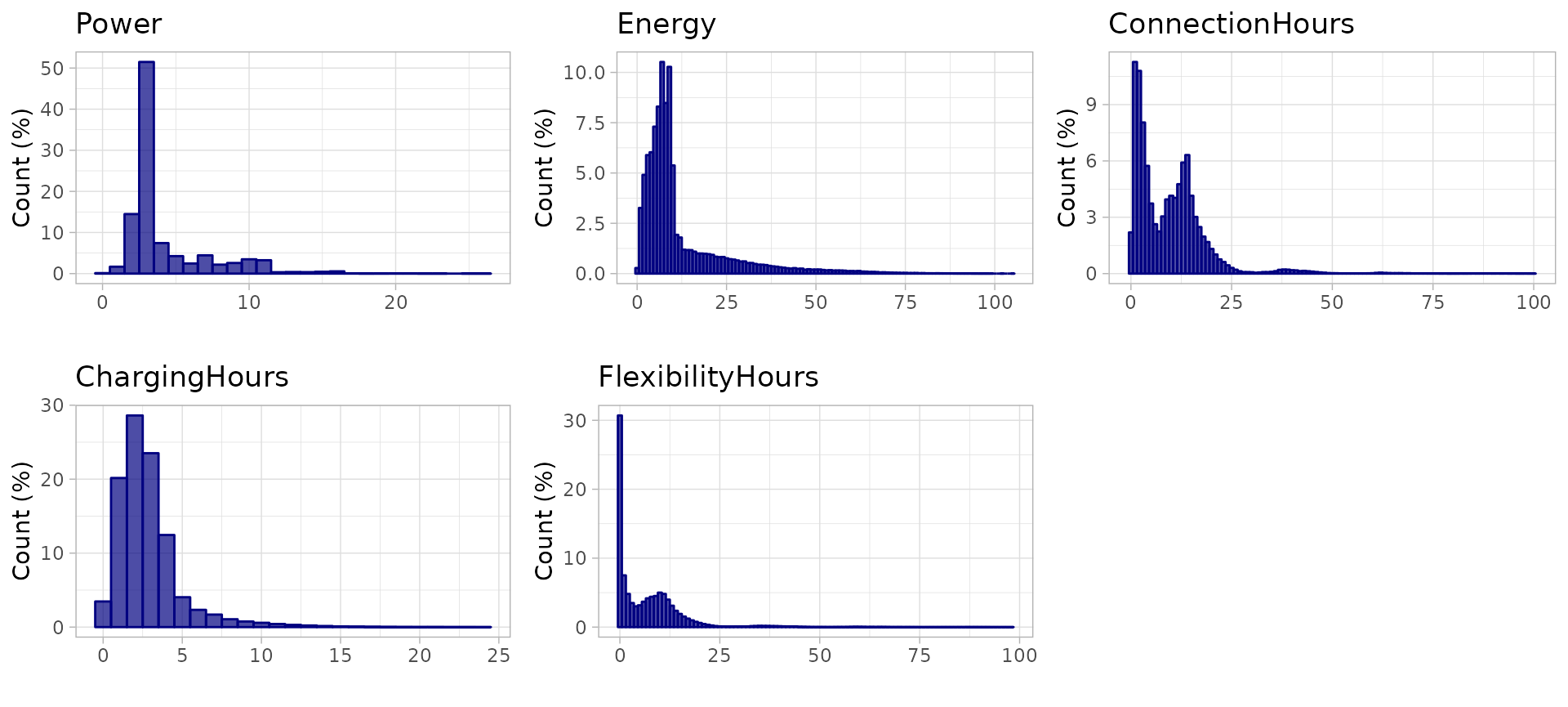
There is no feature that fits a Gaussian distribution, and some
features like ConnectionHours have more than one peak in
the distribution curve. This shows the existence and combination of
different EV user profiles with independent distributions.
Data preprocessing
The clustering method used in package evprof is Gaussian Mixture Models with Expectation-Maximization algorithm, wrapping functions from mclust package. To obtain a better performance in GMM clustering it is important to divide the data in smaller groups and clean the outliers, since the different density distributions will result more accentuated and easy to model.
Divide the data
The division is performed in two steps:
- Disconnection day
- Time-cycle behaviors
Disconnection day division
The different data points groups that stand out from overview plot
correspond to sessions disconnection day. With function
plot_division_lines we can visualize a division from a
certain hour. We will set the division line from 3:00 AM, which means
that sessions below division line disconnect before 3:00 AM of that day,
each line corresponding to a different day.
plot_points(sessions, size = 0.25) %>%
  plot_division_lines(n_lines = 4, division_hour = 3)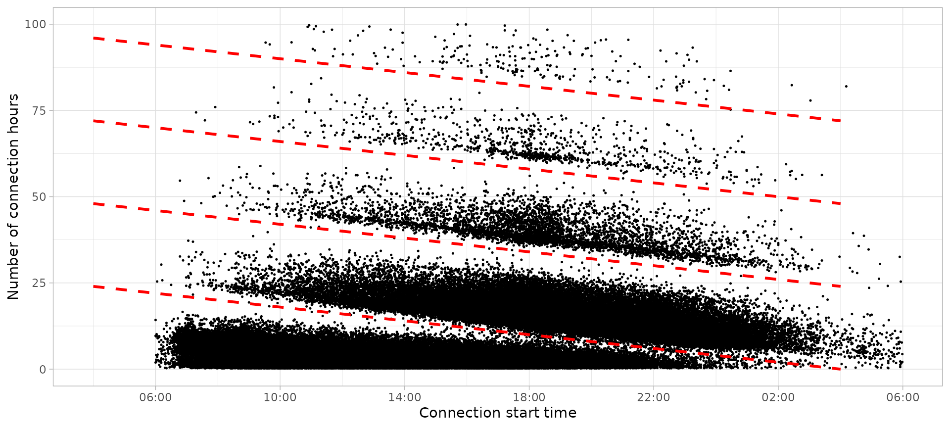
After finding the proper hour to make the division, function
divide_by_disconnection() makes this division adding an
extra column to the data set, Disconnection, with the
number of the corresponding disconnection day. The sessions distribution
over these 5 disconnection days is:
sessions_divisions <- sessions %>%
divide_by_disconnection(division_hour = 3)| Disconnection day | Number of sessions | Percentage of sessions (%) |
|---|---|---|
| 1 | 108109 | 51.31 |
| 2 | 96680 | 45.88 |
| 3 | 4802 | 2.28 |
| 4 | 906 | 0.43 |
| 5 | 214 | 0.10 |
Almost all sessions disconnect the same day or the day after the connection since only 3% of sessions disconnect 2, 3 or 4 days after the connection.
Time-cycle division
It is also important to consider the time-cycles or periods when
users change their behaviors. The function plot_density_2D
lets to analyze the different density of sessions (i.e. users behavior)
according to different weekday, month or year.
plot_density_2D(sessions_divisions, by = 'wday')
plot_density_2D(sessions_divisions, by = 'month')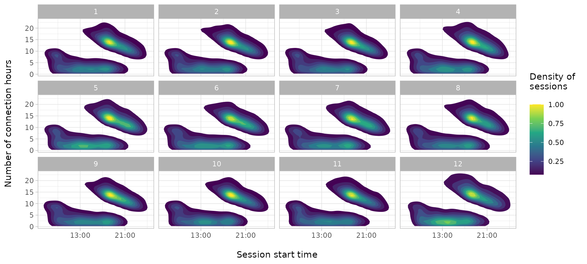
While depending on the weekday the density of sessions is highly
diverse, between months we can’t see a big difference. Moreover, we
could see different distributions on Monday-Thursday, Friday, Saturday
and Sunday, thus we will consider four different groups: working days
(Monday - Thursday), Fridays, Saturdays, Sundays. The division for
time-cycles sessions is performed by function
divide_by_timecycle(), which adds an extra column
Timecycle to the sessions data set with the number of
time-cycle according to function parameters months_cycles
and wdays_cycles.
sessions_divisions <- sessions_divisions %>%
  divide_by_timecycle(
    months_cycles = list(1:12),
    wdays_cycles = list(1:4, 5, 6, 7)
)| Time-cycle | Number of sessions | Percentage of sessions (%) |
|---|---|---|
| 1 | 124533 | 59.10 |
| 2 | 30862 | 14.65 |
| 3 | 30018 | 14.25 |
| 4 | 25298 | 12.01 |
Divided data set
Once the two division approaches are applied, our data set counts
with two extra columns (Disconnection and
Timecycle) to classify each data point within each group.
These columns have integer values corresponding to each division. For a
more readable data set we can change these integer values by character
strings with the definition of each group, and convert them to
factors to set a specific order of the levels.
However, in the Disconnection day division we have seen that sessions disconnecting 2, 3 or 4 days after the connection represent just a 3% of the total data set. Thus, for obtaining generic user profiles these sessions will be discarded. The two Disconnection groups that we will analyze are the sessions that disconnect during the same connection day, labeled as City sessions, and the sessions that disconnect the day after connection, named Home sessions. At the same time, each Time-cycle group has the name of the corresponding weekday: Workday, Friday, Saturday and Sunday.
sessions_divided <- sessions_divisions %>%
  filter(Disconnection %in% c("1", "2")) %>%
  mutate(
    Disconnection = plyr::mapvalues(Disconnection, c("1", "2"), c("City", "Home")),
    Disconnection = factor(Disconnection, levels = c("City", "Home")),
    Timecycle = plyr::mapvalues(Timecycle, c("1", "2", "3", "4"), c("Workday", "Friday", "Saturday", "Sunday")),
    Timecycle = factor(Timecycle, levels = c("Workday", "Friday", "Saturday", "Sunday"))
  )

head(sessions_divided)
Outliers cleaning
As explained, the clustering method used in package
evprof is Gaussian Mixture Models clustering. This method
is sensible to outliers since it tries to explain as most as possible
all the variance of the data. This results to wide and low-precision
Gaussian distributions (clusters). Therefore evprof
package provides different functions to detect and filter outliers. At
the same time, it is also recommended to perform the clustering process
in a logarithmic scale, to include negative values to originally
positive variables. The logarithmic transformation can be done in a lot
of functions setting the log parameter to
TRUE. We can visualize the data of each subset:
plot_points(sessions_divided, size = 0.2, log = T) +
  facet_wrap(vars(Timecycle, Disconnection), scales = 'free', ncol = 4)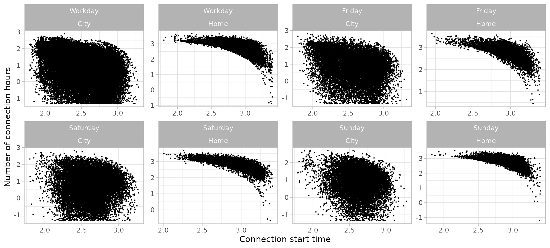
In these plots we see that every group has several points that stand
out from most of points. These outliers can be detected specifying a
noise threshold (in percentage) in function
detect_outliers(). This function adds a logical column
Outlier to the sessions data set showing if a session
whether a session is considered outlier. This classification can be
visualized with function plot_outliers() which shows the
outliers in grey and the noise level (in percentage) in the title of the
graph. This Outlier extra column can be removed together
with outliers with function drop_outliers(). Additionally,
to simply discard sessions from a certain limit in both axis (i.e
connection hours or starting hour), function cut_sessions()
filters the sessions data set according to the specified minimum and
maximum limits of the corresponding axis.
The following plots show the noise-detection process performed for the charging sessions data set and the corresponding filtering, resulting in 8 different clean sub sets ready to be clustered.
Workday city sessions
swc <- sessions_divided %>%
  filter(Disconnection == "City", Timecycle == "Workday") %>%
  cut_sessions(connection_start_min = 1.85, connection_start_max = 3.15, log=T) %>%
  detect_outliers(MinPts = 100, noise_th = 2, log = T)
swc %>% plot_outliers(log = T, size = 0.25)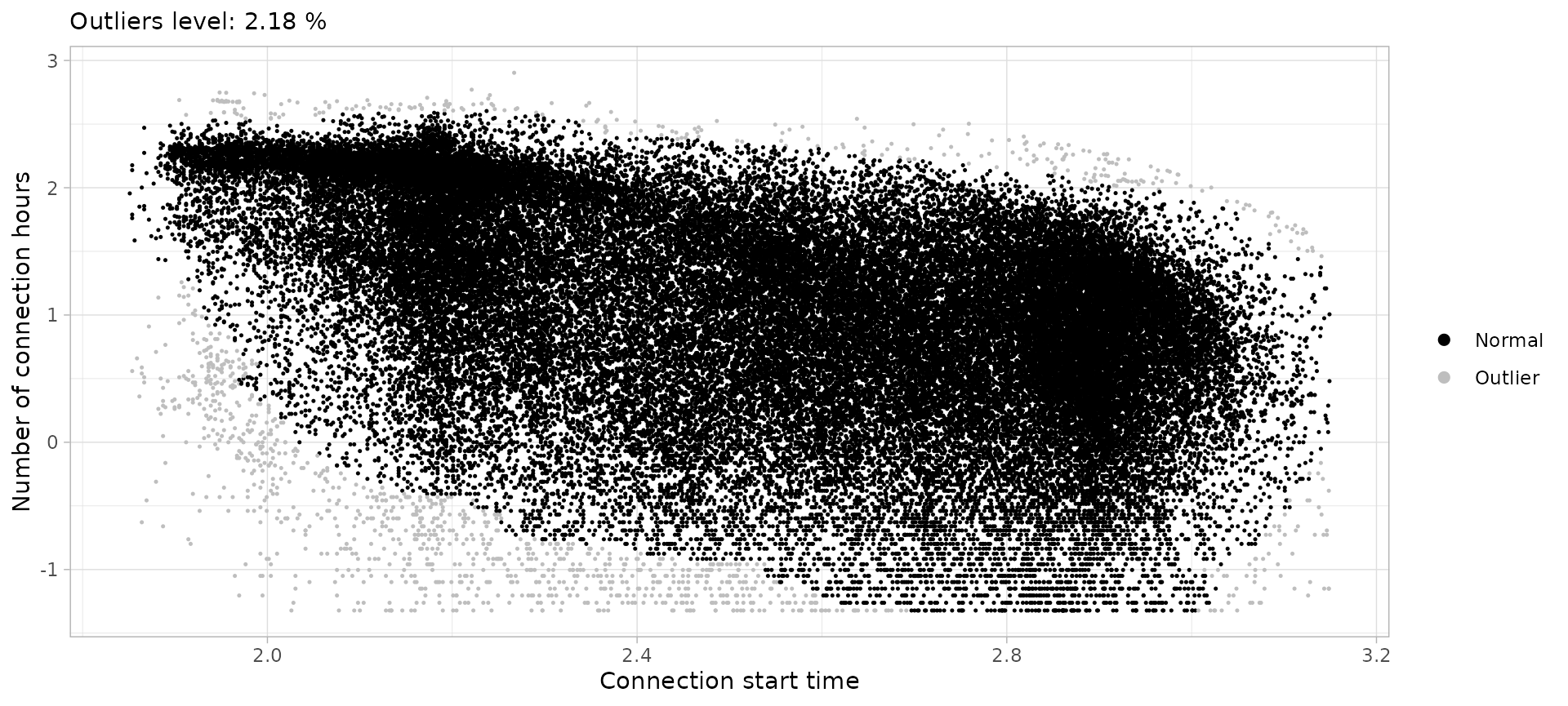
sessions_workday_city <- swc %>%
  drop_outliers()
Workday home sessions
swh <- sessions_divided %>%
  filter(Disconnection == "Home", Timecycle == "Workday") %>%
  cut_sessions(connection_hours_min = 1.5, log=T) %>%
  detect_outliers(MinPts = 200, noise_th = 2, log = T)
swh %>% plot_outliers(log = T, size = 0.25)
sessions_workday_home <- swh %>%
  drop_outliers()
Friday city sessions
sfc <- sessions_divided %>%
  filter(Disconnection == "City", Timecycle == "Friday") %>%
  detect_outliers(MinPts = 50, noise_th = 2, log = T)
sfc %>% plot_outliers(log = T, size = 0.25)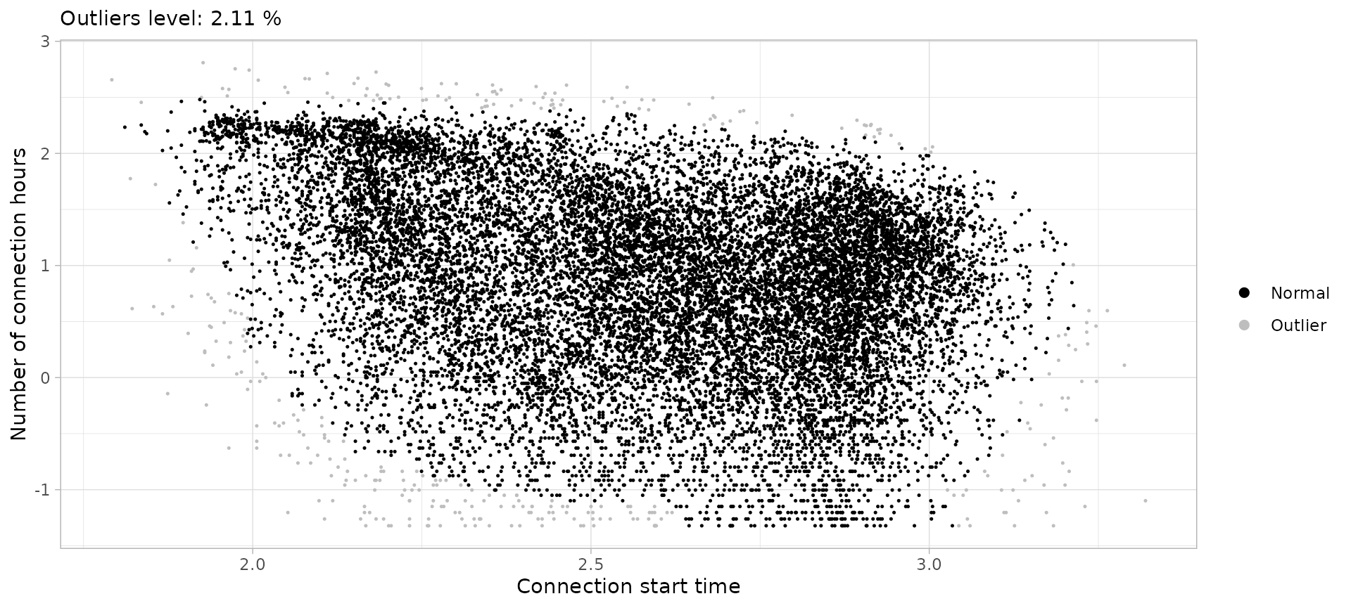
sessions_friday_city <- sfc %>%
  drop_outliers()
Friday home sessions
sfh <- sessions_divided %>%
  filter(Disconnection == "Home", Timecycle == "Friday") %>%
  cut_sessions(connection_hours_min = 1.5, connection_start_min = 2.5, log=T) %>%
  detect_outliers(MinPts = 200, noise_th = 5, log = T)
sfh %>% plot_outliers(log = T, size = 0.25)
sessions_friday_home <- sfh %>%
  drop_outliers()
Saturday city sessions
ssac <- sessions_divided %>%
  filter(Disconnection == "City", Timecycle == "Saturday") %>%
  detect_outliers(MinPts = 200, noise_th = 5, log = T)
ssac %>% plot_outliers(log = T, size = 0.25)
sessions_saturday_city <- ssac %>%
  drop_outliers()
Saturday home sessions
ssah <- sessions_divided %>%
  filter(Disconnection == "Home", Timecycle == "Saturday") %>%
  cut_sessions(connection_hours_min = 1.5, log=T) %>%
  detect_outliers(MinPts = 50, noise_th = 6, log = T)
ssah %>% plot_outliers(log = T, size = 0.25)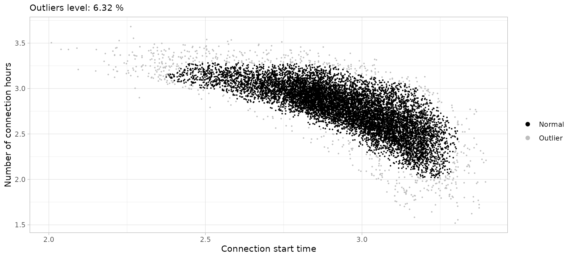
sessions_saturday_home <- ssah %>%
  drop_outliers()
Sunday city sessions
ssuc <- sessions_divided %>%
  filter(Disconnection == "City", Timecycle == "Sunday") %>%
  cut_sessions(connection_start_min = 2.2, log = T ) %>%
  detect_outliers(MinPts = 50, noise_th = 6, log = T)
ssuc %>% plot_outliers(log = T, size = 0.25)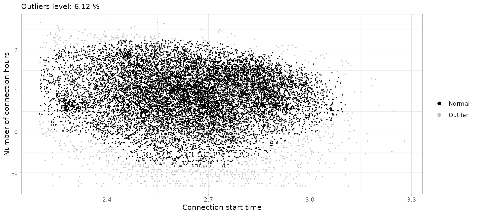
sessions_sunday_city <- ssuc %>%
  drop_outliers()
Sunday home sessions
ssuh <- sessions_divided %>%
  filter(Disconnection == "Home", Timecycle == "Sunday") %>%
  cut_sessions(connection_hours_min = 1.5, connection_start_min = 2.3,
               connection_start_max = 3.25, log = T) %>%
  detect_outliers(MinPts = 200, noise_th = 5, log = T)
ssuh %>% plot_outliers(log = T, size = 0.25)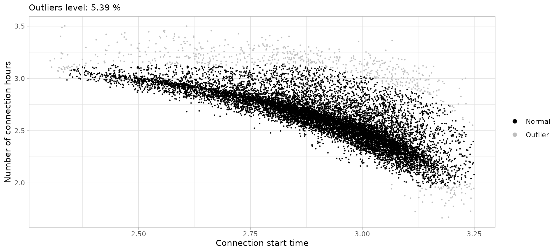
sessions_sunday_home <- ssuh %>%
  drop_outliers()
Clustering process
Function cluster_sessions perform a classification of
sessions adding an extra column Cluster with the
corresponding cluster number. However, Gaussian Mixture Models need a
predefined number of clusters k. Moreover, this function
also requires a seed in order to define a specific random
seed and being able to reproduce specifics clustering results.
Parameters selection
The Bayesan Information Criterion (BIC) is a common approach to find the optimal number of clusters to consider for the GMM clustering. BIC values are an approximation to intergrated likelihood (explained variance in data) with a penalty on the number of components, so the ‘best’ model is the one with the highest BIC among the fitted models.
To evaluate the BIC of your data sets according to the number of
components use function choose_k_GMM(), for example:
choose_k_GMM(sessions_workday_city, k = 3:10, log = T)After generating a BIC plot for each one of the 8 sub-sets, the selected number of clusters are:
- Sessions workday city:
k = 6 - Sessions workday home:
k = 6 - Sessions Friday city:
k = 6 - Sessions Friday home:
k = 6 - Sessions Saturday city:
k = 5 - Sessions Saturday home:
k = 5 - Sessions Sunday city:
k = 5 - Sessions Sunday home:
k = 6
Then, since Gaussian Mixture Modeling depends on the random seed of
the operation, it is recommended to repeat the clustering process
several times and observe the variability. If different clusters are
obtained in each repetition, it means that there is still too much noise
or variance in the data, or that a different number of clusters should
be selected. Function save_clustering_iterations() repeats
the clustering the number of times specified in the it
parameter and saves the results in a PDF file. From this file, then we
can choose the optimal seed according to the BIC value. For example:
save_clustering_iterations(
  sessions_workday_city, k=6, it=6, log = T,
  filename = "figures/clusters/workday_city_k-6.pdf"
)
For this study case, each data sub-set has been clustered 6 times and the optimal seeds for each sub-set have resulted as follows:
- Sessions Workday city:
seed = 91 - Sessions Workday home:
seed = 643 - Sessions Friday city:
seed = 311 - Sessions Friday home:
seed = 436 - Sessions Saturday city:
seed = 668 - Sessions Saturday home:
seed = 537 - Sessions Sunday city:
seed = 908 - Sessions Sunday home:
seed = 566
Clustering
Finally, we can cluster each sub-set with function
cluster_sessions(), specifying the parameters
k and seed with the corresponding values
previously found:
workday_city_GMM <- cluster_sessions(
sessions_workday_city, k = 6, seed = 91, log = T
)
workday_home_GMM <- cluster_sessions(
sessions_workday_home, k = 6, seed = 643, log = T
)
friday_city_GMM <- cluster_sessions(
sessions_friday_city, k = 6, seed = 311, log = T
)
friday_home_GMM <- cluster_sessions(
sessions_friday_home, k = 6, seed = 436, log = T
)
saturday_city_GMM <- cluster_sessions(
sessions_saturday_city, k = 5, seed = 668, log = T
)
saturday_home_GMM <- cluster_sessions(
sessions_saturday_home, k = 6, seed = 92, log = T
)
sunday_city_GMM <- cluster_sessions(
sessions_sunday_city, k = 5, seed = 101, log = T
)
sunday_home_GMM <- cluster_sessions(
sessions_sunday_home, k = 6, seed = 191, log = T
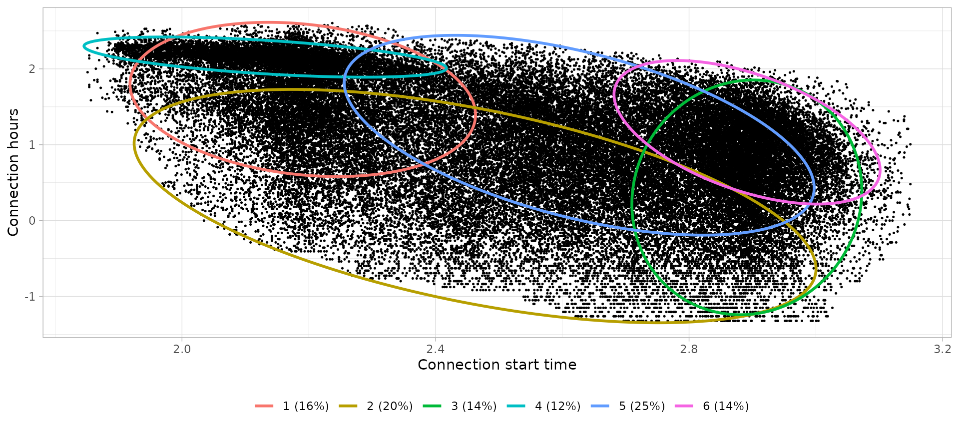
)The object returned by cluster_sessions() function is a
list with two other objects:
-
sessions: atibblecontaining the sessions’ data set with an extra columnCluster(i.e. the corresponding cluster number) -
models: atibblewith the means and co-variance matrix of each cluster’s Gaussian Mixture Models
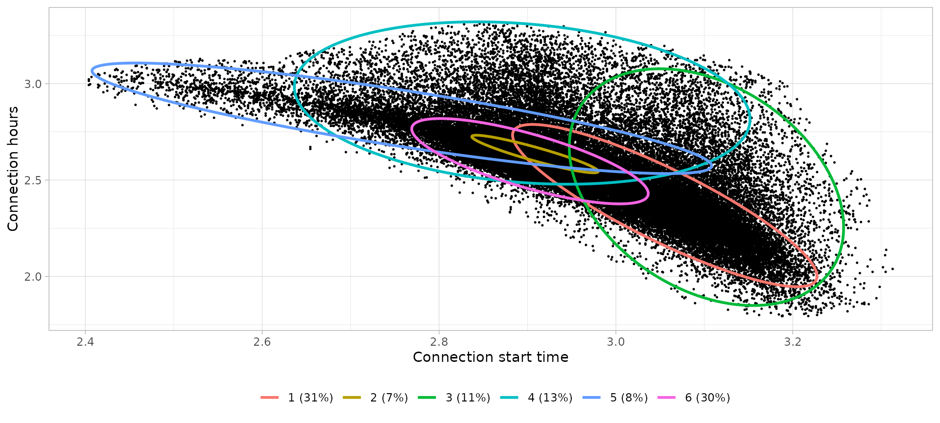
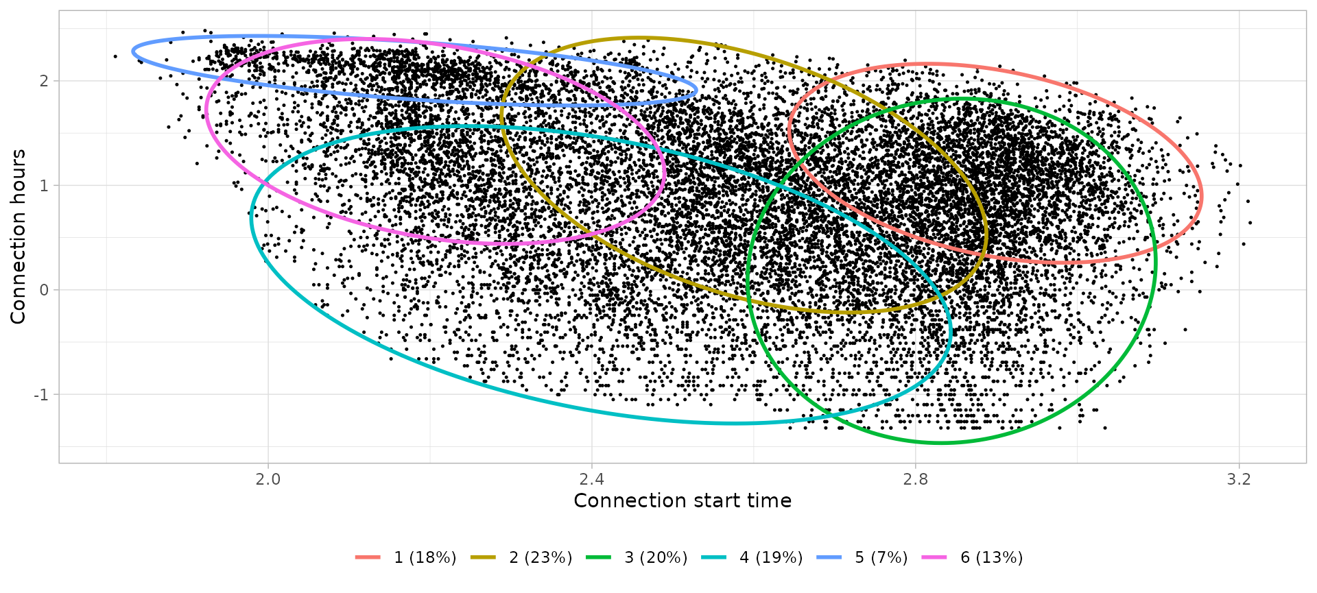
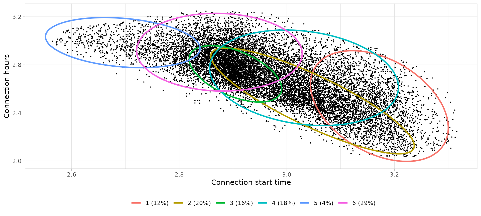
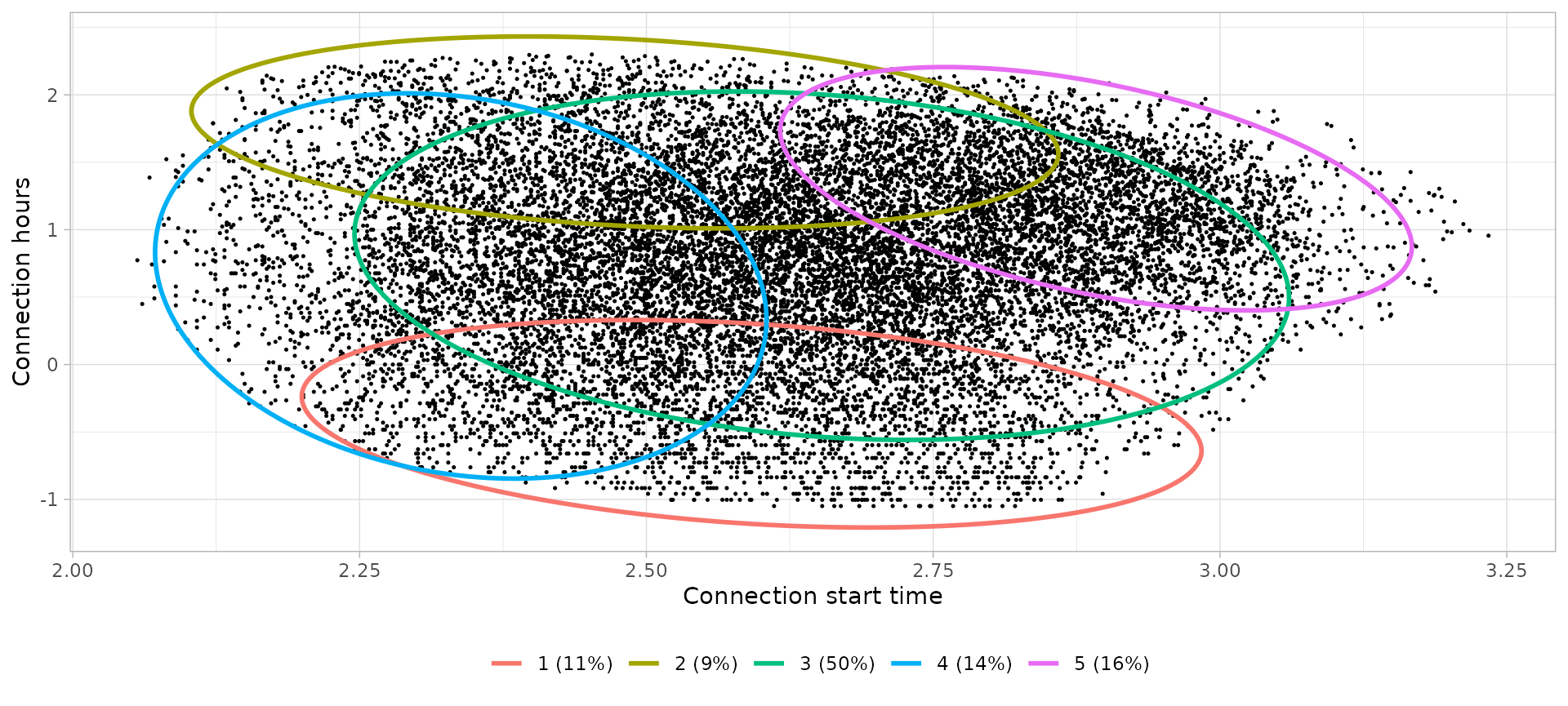
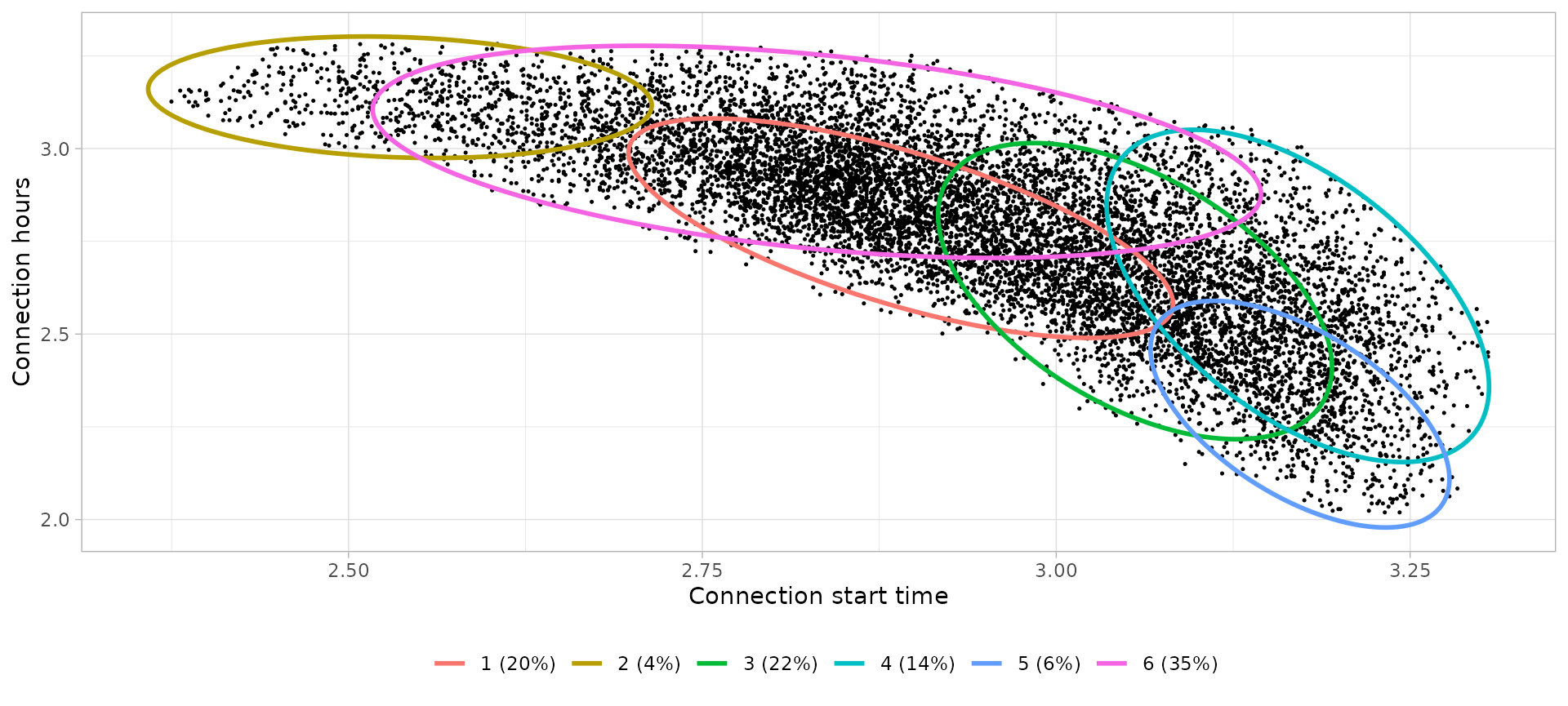
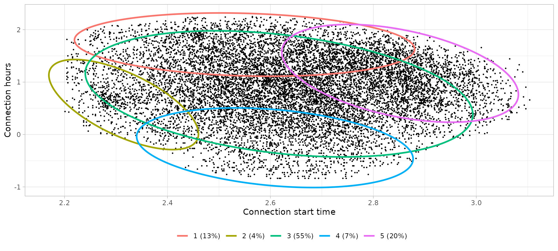
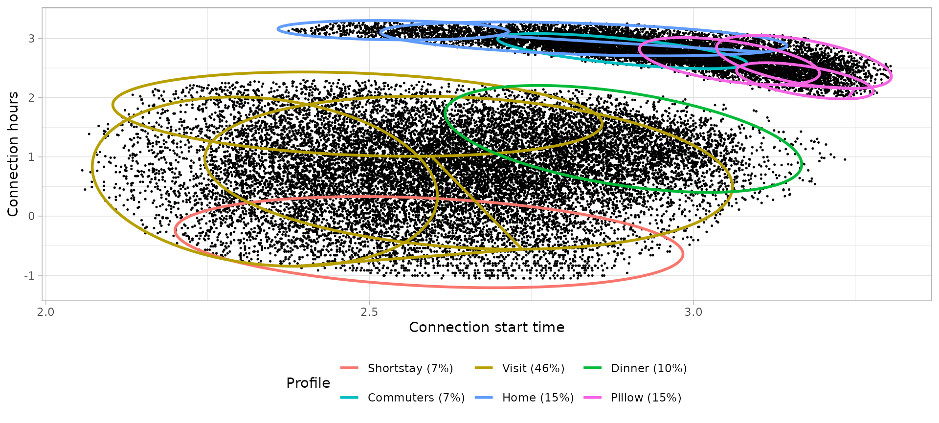
These two objects correspond to the parameters sessions
and models of the function plot_bivarGMM(),
which plots each cluster as an ellipse over the sessions’ points. For
example:
workday_city_bivarGMM_plot <- plot_bivarGMM(
  sessions = workday_city_GMM$sessions,
  models = workday_city_GMM$models,
  profiles_names = paste0(
    workday_city_GMM$models$cluster,
    " (", round(workday_city_GMM$models$ratio*100), "%)"
  ),
  log = T, legend_nrow = 1
)
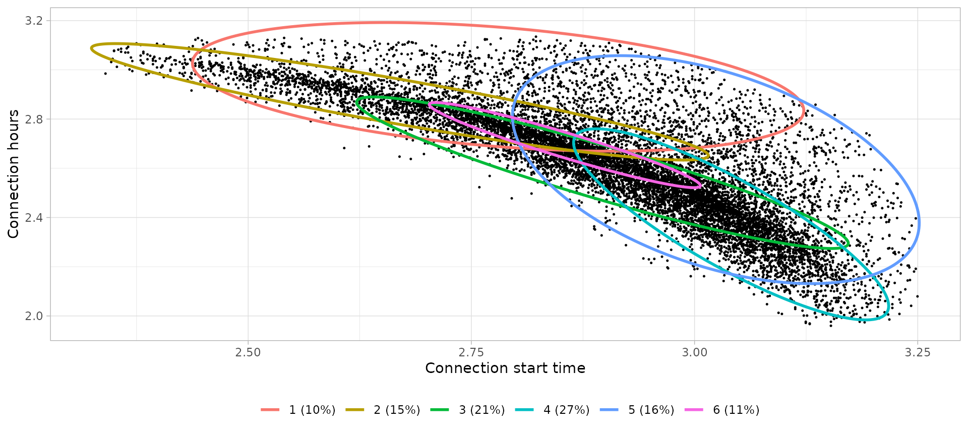
Using purrr iteration we can generate a list with a plot
for each sub-set.
bivarGMM_plots <- purrr::map2(
list(
workday_city_GMM$sessions, workday_home_GMM$sessions,
friday_city_GMM$sessions, friday_home_GMM$sessions,
saturday_city_GMM$sessions, saturday_home_GMM$sessions,
sunday_city_GMM$sessions, sunday_home_GMM$sessions
),
list(
workday_city_GMM$models, workday_home_GMM$models,
friday_city_GMM$models, friday_home_GMM$models,
saturday_city_GMM$models, saturday_home_GMM$models,
sunday_city_GMM$models, sunday_home_GMM$models
),
~ plot_bivarGMM(
.x, .y,
profiles_names = paste0(.y$cluster, " (", round(.y$ratio*100), "%)"),
log = T,
legend_nrow = 1
)
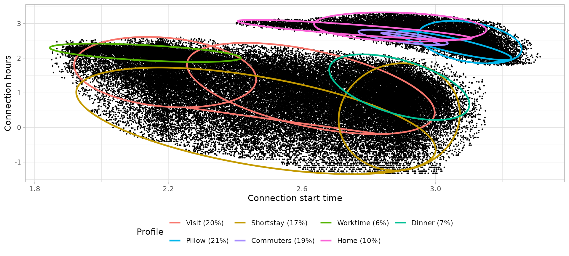
)We will visualize the clusters of each subsets in Profiling section, together with the interpretation of each cluster and the corresponding assignation to a user profile.
Profiling
Clusters obtained from GMM don’t give a lot of information themselves and separately may have an unclear meaning. In this section we will define each cluster to give them a meaning and relate them to generic user behaviors, i.e. user profiles. Moreover, not every clusters must correspond to a single user profile, clusters with the same or a similar meaning can be grouped to a user profile. Thus, the combination of these multiple Gaussian Mixture Models into a single user profile is what we expect to result in a daily generic behavior of EV users.
As a tool to define the different clusters, function
define_clusters() prints the average value of the
connection start time and connection duration (i.e. the centroid) of
each cluster. If the cluster process was performed in logarithmic scale,
these values are transformed to natural scale for a better
understanding. Moreover, we can pass to the parameters
interpretations and profile_names a list of
character strings with the corresponding interpretation of the centroids
(e.g. “Connection after work-time, leaving always next morning”) and the
user profile name assigned to each interpretation (e.g. “Commuter”).
Workdays
Workday city

# Define clusters
workday_city_clusters_profiles <- define_clusters(
  models = workday_city_GMM$models,
  interpretations = c(
    "Visits during the morning or whole day",
    "Short visits during the day",
    "Short visits during the evening",
    "Full-day working time",
    "Visits during the afternoon",
    "Dinner time"
  ),
  profile_names = c(
    "Visit",
    "Shortstay",
    "Shortstay",
    "Worktime",
    "Visit",
    "Dinner"
  ),
  log = T
)

workday_city_clusters_profiles %>%
  knitr::kable(digits = 2, col.names = c(
    "Cluster", "Controid Start time", "Centroid Connection hours",
    "Interpretation", "Profile"
))| Cluster | Controid Start time | Centroid Connection hours | Interpretation | Profile |
|---|---|---|---|---|
| 1 | 08:56 | 4.94 | Visits during the morning or whole day | Visit |
| 2 | 11:44 | 1.21 | Short visits during the day | Shortstay |
| 3 | 18:01 | 1.36 | Short visits during the evening | Shortstay |
| 4 | 08:26 | 8.63 | Full-day working time | Worktime |
| 5 | 13:50 | 3.08 | Visits during the afternoon | Visit |
| 6 | 18:01 | 3.20 | Dinner time | Dinner |
Workday home
# Define clusters
workday_home_clusters_profiles <- define_clusters(
  models = workday_home_GMM$models,
  interpretations = c(
    "Connection during the night, leaving next morning",
    "Connection after work, leaving next morning",
    "Connection during the night, not necessarily leaving next morning",
    "Connection during the afternoon, not necessarily leaving next morning",
    "Connection during the afternoon, leaving next morning",
    "Connection after work, leaving next morning"
  ),
  profile_names = c(
    "Pillow",
    "Commuters",
    "Pillow",
    "Home",
    "Home",
    "Commuters"
  ),
  log = T
)

workday_home_clusters_profiles %>%
  knitr::kable(digits = 2, col.names = c(
    "Cluster", "Controid Start time", "Centroid Connection hours",
    "Interpretation", "Profile"
))| Cluster | Controid Start time | Centroid Connection hours | Interpretation | Profile |
|---|---|---|---|---|
| 1 | 21:14 | 10.67 | Connection during the night, leaving next morning | Pillow |
| 2 | 18:20 | 13.95 | Connection after work, leaving next morning | Commuters |
| 3 | 22:15 | 11.74 | Connection during the night, not necessarily leaving next morning | Pillow |
| 4 | 18:04 | 18.17 | Connection during the afternoon, not necessarily leaving next morning | Home |
| 5 | 15:46 | 16.79 | Connection during the afternoon, leaving next morning | Home |
| 6 | 18:14 | 13.44 | Connection after work, leaving next morning | Commuters |
Fridays
Friday city
# Define clusters
friday_city_clusters_profiles <- define_clusters(
  models = friday_city_GMM$models,
  interpretations = c(
    "Dinner time",
    "Visits during the afternoon",
    "Short visits during the evening",
    "Short visits during the day",
    "Full-day working time",
    "Visits during the morning or whole day"
  ),
  profile_names = c(
    "Dinner",
    "Visit",
    "Shortstay",
    "Shortstay",
    "Worktime",
    "Visit"
  ),
  log = T
)

friday_city_clusters_profiles %>%
  knitr::kable(digits = 2, col.names = c(
    "Cluster", "Controid Start time", "Centroid Connection hours",
    "Interpretation", "Profile"
))| Cluster | Controid Start time | Centroid Connection hours | Interpretation | Profile |
|---|---|---|---|---|
| 1 | 18:09 | 3.36 | Dinner time | Dinner |
| 2 | 13:18 | 3.00 | Visits during the afternoon | Visit |
| 3 | 17:12 | 1.20 | Short visits during the evening | Shortstay |
| 4 | 11:09 | 1.15 | Short visits during the day | Shortstay |
| 5 | 08:51 | 8.14 | Full-day working time | Worktime |
| 6 | 09:05 | 4.14 | Visits during the morning or whole day | Visit |
Friday home
# Define clusters
friday_home_clusters_profiles <- define_clusters(
  models = friday_home_GMM$models,
  interpretations = c(
    "Connection during the night, not necessarily leaving next morning",
    "Connection during the night, leaving during next morning",
    "Connection after work, leaving during next morning",
    "Connection during the night, not necessarily leaving next morning",
    "Connection during the afternoon, leaving next morning",
    "Connection during the afternoon, not necessarily leaving next morning"
  ),
  profile_names = c(
    "Pillow",
    "Pillow",
    "Commuters",
    "Pillow",
    "Home",
    "Home"
  ),
  log = T
)

friday_home_clusters_profiles %>%
  knitr::kable(digits = 2, col.names = c(
  "Cluster", "Controid Start time", "Centroid Connection hours",
  "Interpretation", "Profile"
))| Cluster | Controid Start time | Centroid Connection hours | Interpretation | Profile |
|---|---|---|---|---|
| 1 | 23:51 | 11.67 | Connection during the night, not necessarily leaving next morning | Pillow |
| 2 | 21:04 | 12.18 | Connection during the night, leaving during next morning | Pillow |
| 3 | 18:15 | 15.25 | Connection after work, leaving during next morning | Commuters |
| 4 | 20:44 | 14.76 | Connection during the night, not necessarily leaving next morning | Pillow |
| 5 | 14:48 | 19.78 | Connection during the afternoon, leaving next morning | Home |
| 6 | 17:43 | 18.26 | Connection during the afternoon, not necessarily leaving next morning | Home |
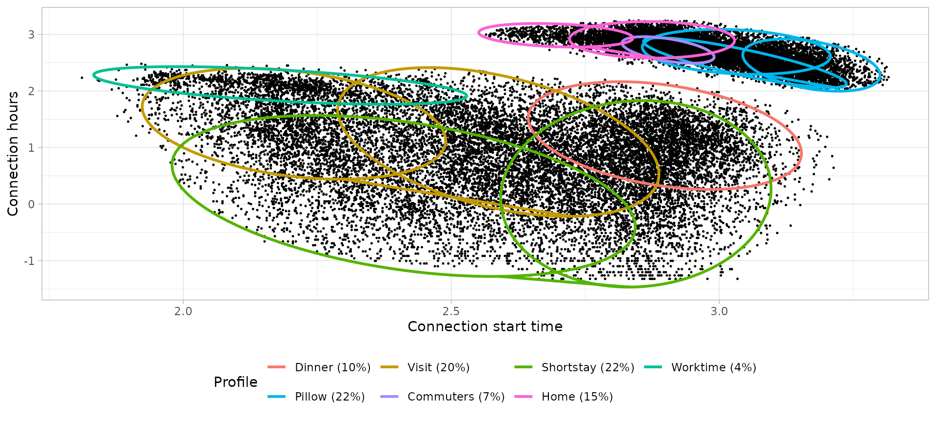
Notes:
- The Friday Home cluster that leave next day is not so narrow (concentrated) than Workday Home cluster since people has no timetable on weekends morning.
- The Commuter profile on Fridays is different than Workdays Commuter since the after-work sessions are more dispersed in terms of both starting time and duration. This could be a result of not working on Friday afternoon (or leave early from work) and not having to leave early next morning.
Saturdays
Saturday city
# Define clusters
saturday_city_clusters_profiles <- define_clusters(
  models = saturday_city_GMM$models,
  interpretations = c(
    "Short visits during the day",
    "Visits during the day",
    "Visits during the afternoon",
    "Visits during the morning",
    "Dinner time"
  ),
  profile_names = c(
    "Shortstay",
    "Visit",
    "Visit",
    "Visit",
    "Dinner"
  ),
  log = T
)

saturday_city_clusters_profiles %>%
  knitr::kable(digits = 2, col.names = c(
    "Cluster", "Controid Start time", "Centroid Connection hours",
    "Interpretation", "Profile"
))| Cluster | Controid Start time | Centroid Connection hours | Interpretation | Profile |
|---|---|---|---|---|
| 1 | 13:21 | 0.64 | Short visits during the day | Shortstay |
| 2 | 11:57 | 5.59 | Visits during the day | Visit |
| 3 | 14:12 | 2.08 | Visits during the afternoon | Visit |
| 4 | 10:22 | 1.79 | Visits during the morning | Visit |
| 5 | 18:02 | 3.68 | Dinner time | Dinner |
Notes:
- Shortstay profile is in minority during Saturdays in favour to Visit profile, probably because people have time to make longer visits rather than short ones.
Saturday home
# Define clusters
saturday_home_clusters_profiles <- define_clusters(
  models = saturday_home_GMM$models,
  interpretations = c(
    "Connection during the noon, leaving next morning",
    "Connection during the early-afternoon, leaving next morning",
    "Connection during the night, leaving next morning",
    "Connection during the night, not necessarily leaving next morning",
    "Connection during the night, leaving next morning",
    "Connection during the afternoon, not necessarily leaving next morning"
  ),
  profile_names = c(
    "Commuters",
    "Home",
    "Pillow",
    "Pillow",
    "Pillow",
    "Home"
  ),
  log = T
)

saturday_home_clusters_profiles %>%
  knitr::kable(digits = 2, col.names = c(
    "Cluster", "Controid Start time", "Centroid Connection hours",
    "Interpretation", "Profile"
))| Cluster | Controid Start time | Centroid Connection hours | Interpretation | Profile |
|---|---|---|---|---|
| 1 | 18:00 | 16.21 | Connection during the noon, leaving next morning | Commuters |
| 2 | 12:38 | 23.07 | Connection during the early-afternoon, leaving next morning | Home |
| 3 | 21:14 | 13.68 | Connection during the night, leaving next morning | Pillow |
| 4 | 23:49 | 13.50 | Connection during the night, not necessarily leaving next morning | Pillow |
| 5 | 23:52 | 9.82 | Connection during the night, leaving next morning | Pillow |
| 6 | 16:58 | 19.91 | Connection during the afternoon, not necessarily leaving next morning | Home |
Notes:
- The Friday Home cluster that leave next day is not so narrow (concentrated) than Workday Home cluster since people has no timetable on weekends morning. The weekends user profiles are more variable and less clear.
- On weekends we don’t have commuters since they don’t go from work to home, thus the afternoon sessions belong now to Home profile.
Sundays
Sunday city
# Define clusters
sunday_city_clusters_profiles <- define_clusters(
  models = sunday_city_GMM$models,
  interpretations = c(
    "Visits during the morning or whole day",
    "Visits during the morning",
    "Visits during the day",
    "Short visits during the day",
    "Dinner time"
  ),
  profile_names = c(
    "Visit",
    "Visit",
    "Visit",
    "Shortstay",
    "Dinner"
  ),
  log = T
)

sunday_city_clusters_profiles %>%
  knitr::kable(digits = 2, col.names = c(
    "Cluster", "Controid Start time", "Centroid Connection hours",
    "Interpretation", "Profile"
))| Cluster | Controid Start time | Centroid Connection hours | Interpretation | Profile |
|---|---|---|---|---|
| 1 | 12:48 | 5.56 | Visits during the morning or whole day | Visit |
| 2 | 10:07 | 1.77 | Visits during the morning | Visit |
| 3 | 13:41 | 2.17 | Visits during the day | Visit |
| 4 | 13:35 | 0.78 | Short visits during the day | Shortstay |
| 5 | 17:19 | 3.21 | Dinner time | Dinner |
Notes:
- Shortstay visits are less relevant during the Sunday since the shops or places to make short assignments are closed on this weekday.
- The Dinner profile has more weight here (20%) than the other time-cycles (around 15%)
Sunday home
# Define clusters
sunday_home_clusters_profiles <- define_clusters(
  models = sunday_home_GMM$models,
  interpretations = c(
    "Connection during the afternoon, not necessarily leaving next morning",
    "Connection during the afternoon, leaving next morning",
    "Connection during the afternoon, leaving next morning",
    "Connection during the night, leaving next morning",
    "Connection during the night, not necessarily leaving next morning",
    "Connection during the afternoon, leaving next morning"
  ),
  profile_names = c(
    "Home",
    "Home",
    "Commuters",
    "Pillow",
    "Pillow",
    "Commuters"
  ),
  log = T
)

sunday_home_clusters_profiles %>%
  knitr::kable(digits = 2, col.names = c(
    "Cluster", "Controid Start time", "Centroid Connection hours",
    "Interpretation", "Profile"
))| Cluster | Controid Start time | Centroid Connection hours | Interpretation | Profile |
|---|---|---|---|---|
| 1 | 16:07 | 18.74 | Connection during the afternoon, not necessarily leaving next morning | Home |
| 2 | 14:26 | 17.64 | Connection during the afternoon, leaving next morning | Home |
| 3 | 18:07 | 13.22 | Connection during the afternoon, leaving next morning | Commuters |
| 4 | 20:56 | 10.72 | Connection during the night, leaving next morning | Pillow |
| 5 | 20:34 | 13.39 | Connection during the night, not necessarily leaving next morning | Pillow |
| 6 | 17:22 | 14.80 | Connection during the afternoon, leaving next morning | Commuters |
Notes:
- Here we have again a narrow afternoon Home clusters that show people leaving next morning since Monday is a working day.
- On weekends we don’t have commuters since they don’t go from work to home.
Sessions classification into user profiles
After assigning a user profile to each cluster through the clusters
definitions with function define_clusters(), we can use the
data frame that this function outputs as the
clusters_definition parameter of function
set_profiles(). This function wraps all sub-sets sessions
and clusters definitions to return a total sessions data set with an
extra Profile column, finishing with this function the user
profile classification of the charging sessions data set. The other
parameter that function set_profiles() needs is the
sessions_clustered, which is the sessions
object from the output of cluster_sessions function.
# Join the classification of each subset
sessions_profiles <- set_profiles(
  sessions_clustered = list(
    workday_city_GMM$sessions, workday_home_GMM$sessions,
    friday_city_GMM$sessions, friday_home_GMM$sessions,
    saturday_city_GMM$sessions, saturday_home_GMM$sessions,
    sunday_city_GMM$sessions, sunday_home_GMM$sessions
  ),
  clusters_definition = list(
    workday_city_clusters_profiles, workday_home_clusters_profiles,
    friday_city_clusters_profiles, friday_home_clusters_profiles,
    saturday_city_clusters_profiles, saturday_home_clusters_profiles,
    sunday_city_clusters_profiles, sunday_home_clusters_profiles
  )
)

head(sessions_profiles)
## # A tibble: 6 × 15
## Profile Session ConnectionStartDateTime ConnectionEndDateTime
## <chr> <chr> <dttm> <dttm>
## 1 Shortstay 86437 2015-09-02 07:35:00 2015-09-02 09:02:00
## 2 Worktime 86444 2015-09-02 07:46:00 2015-09-02 15:39:00
## 3 Worktime 86450 2015-09-02 08:00:00 2015-09-02 17:55:00
## 4 Visit 86466 2015-09-02 08:38:00 2015-09-02 11:49:00
## 5 Visit 86486 2015-09-02 08:58:00 2015-09-02 13:11:00
## 6 Worktime 86492 2015-09-02 09:07:00 2015-09-02 17:33:00
## # ℹ 11 more variables: ChargingStartDateTime <dttm>,
## # ChargingEndDateTime <dttm>, Power <dbl>, Energy <dbl>,
## # ConnectionHours <dbl>, ChargingHours <dbl>, FlexibilityHours <dbl>,
## # ChargingStation <chr>, Disconnection <fct>, Timecycle <fct>, Cluster <chr>To visualize the classification we can plot the charging sessions points with a different color for every user profile, and separate between time-cycle.
classification_profiles_plot <-
  plot_points(
    sessions_profiles, start = 6, log = FALSE,
    aes(color = Profile), size = 0.3
  ) +
  facet_wrap(vars(Timecycle)) +
  guides(colour = guide_legend(override.aes = list(size=2)))

classification_profiles_plot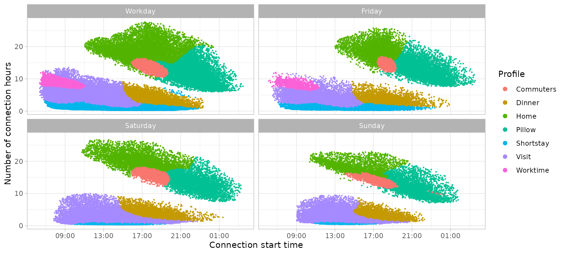
Although the same user profiles names are used in all time-cycles, we can appreciate some differences that support our approach to make a model for each time-cycle independently:
- Worktime sessions appear with a clear shape only during working days, while on weekends the morning sessions are more variable and have been assigned to the Visit user profile. The Worktime sessions on Friday are the half of Worktime sessions on any other working day.
- Short-stay sessions are in minority during Weekends days since we have longer sessions instead, or some business places are closed.
- The Home profile present narrower cluster shapes when the next day is a working day (Workday and Sunday time-cycles). When users don’t have a defined timetable the following day, sessions are more variable in terms of both duration and start time.
- Dinner profile has more importance during Sundays than the other time-cycles.
To conclude the profiling section, we could summarize the user profiles with the following classification based on their connections features:
-
Specific profiles: all sessions have similar start
time and connection duration
- Worktime: connections start between 8:00 and 9:00, with a duration of 8-9 hours.
- Commuters: connections start between 18:00 and 19:00, with a duration of 13-14 hours (leaving between 7:00-8:00 of next day)
- Diner: connections start between 18:00 and 19:00, with a duration of 3-4 hours.
-
Semi-specific profiles: sessions have similar start
time or connection duration.
- Shortstay: connection duration of 1.5 hours in average.
- Pillow: connection start time from 21:00.
-
Variable profiles: sessions with a wide range of
start time and connection duration values
- Visit: city sessions that start during all day with a variety of short and long connection duration.
- Home: home sessions that start during all afternoon not necessarily leaving next day.
User profiles modelling
As seen before, we have divided the data in two subsets considering the time-cycles where EV user profiles change their behaviors. In this case we have four different time cycles: Workdays, Fridays, Saturdays and Sundays.
Each time-cycle has its own connection models
(connection start time and duration) based on the Gaussian Mixture
Models corresponding to every user profile. However, to estimate new
charging sessions we need to model the energy required
as well. The energy consumed is very sensitive to latest models of EV in
the market, since the batteries and charging rates are larger with every
new model. To deal with this variability, it is recommended to build
energy models using the most recent data in the data set. Moreover, the
energy models should be done separately according to the
Power charging rate, since this is a determinant variable
for the value of energy charged.
Each time-cycle model will be stored in tibbles with the
following variables:
-
profile: Character vector with profiles names. Each profile is a row in the tibble. -
profile_ratio: Numeric vector with the ratio or percentage of sessions corresponding to each profile for this time cycle, obtained from functionget_connection_models(). In case of modifying these ratios, their values must be always between 0 and 1. -
connection_models: List of tibbles containing the connection models of each profile, obtained from functionget_connection_models(). -
energy_models: List of tibbles containing the energy models of each profile, obtained from functionget_energy_models().
On one hand, after obtaining the connection models (i.e. bi-variate
Gaussian Mixture Models weights, means and co-variance matrices) with
function get_connection_models(), we can visualize them
with function plot_model_clusters() which outputs a similar
ellipses plot than function plot_bivarGMM() but using a
different color for each user profile instead of clusters (the clusters
of a same profile have the same color now).
On the other hand, the energy models (i.e. uni-variate Gaussian
Mixture Models weights, means and variance) obtained with function
get_energy_models() can be visualized with function
plot_energy_models_density(). We will create an energy
model for every different charging rate in Power column of
the data set. Therefore, to avoid overfitting, the Power
value of all sessions has to be rounded to the three most common values
in the charging infrastructure: 3.7 kW, 7.4 kW and 11 kW.
sessions_energy_models <- sessions_profiles %>%
  filter(
    lubridate::year(ConnectionStartDateTime) == 2020,
    lubridate::month(ConnectionStartDateTime) < 3
  ) %>%
  mutate(
    Power = round_to_interval(Power, 3.7)
  )
sessions_energy_models$Power[sessions_energy_models$Power == 0] <- 3.7
sessions_energy_models$Power[sessions_energy_models$Power > 11] <- 11
Workdays models
Connection models: Bi-variate Gaussian Mixture Models
# Build the models
workday_connection_models <- get_connection_models(
  subsets_clustering = list(
    workday_city_GMM, workday_home_GMM
  ),
  clusters_definition = list(
    workday_city_clusters_profiles, workday_home_clusters_profiles
  )
)
# Plot the bivariate GMM
workday_connection_models_plot <- plot_model_clusters(
  subsets_clustering = list(
    workday_city_GMM, workday_home_GMM
  ),
  clusters_definition = list(
    workday_city_clusters_profiles, workday_home_clusters_profiles
  ),
  profiles_ratios = workday_connection_models[c("profile", "ratio")],
  log = TRUE
)
Energy models: Uni-variate Gaussian Mixture Models
# Build the models
workday_energy_models <- sessions_energy_models %>%
  filter(Timecycle == 'Workday') %>%
  get_energy_models(
    log = TRUE,
    by_power = TRUE
  )
# Plot the univariate GMM
workday_energy_models_plots <- plot_energy_models(workday_energy_models)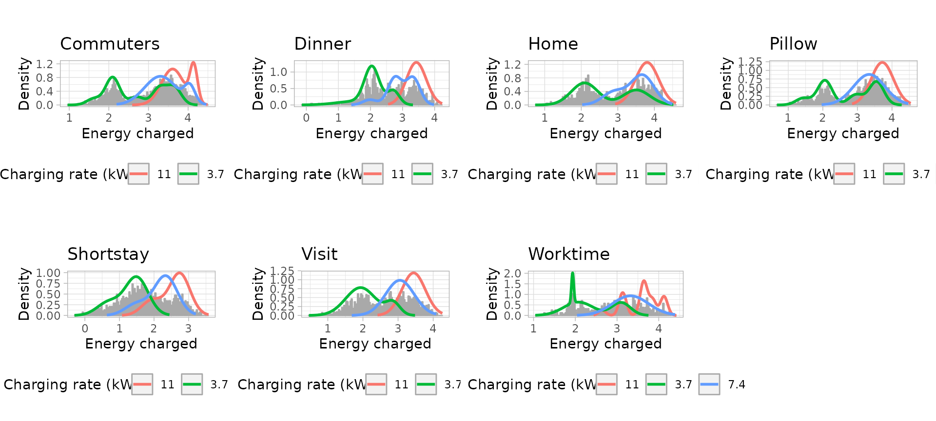
Fridays models
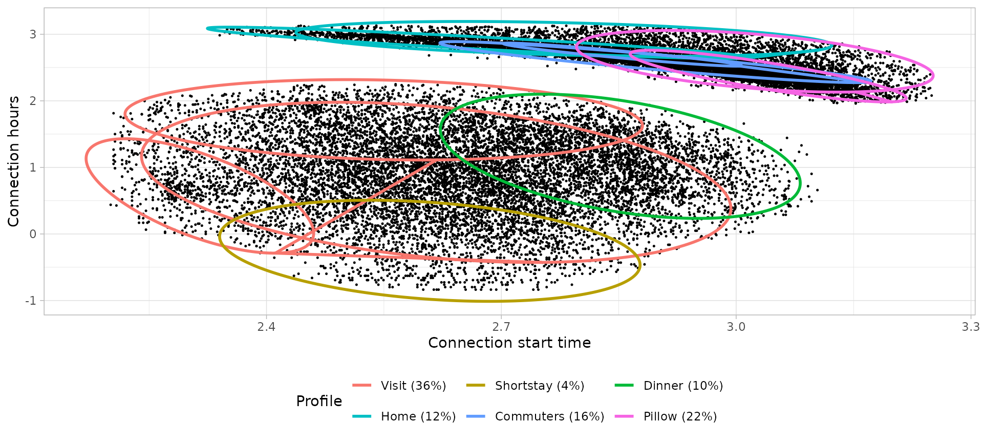
Connection models: Bi-variate Gaussian Mixture Models
# Build the models
friday_connection_models <- get_connection_models(
  subsets_clustering = list(
    friday_city_GMM, friday_home_GMM
  ),
  clusters_definition = list(
    friday_city_clusters_profiles, friday_home_clusters_profiles
  )
)
# Plot the bivariate GMM
friday_connection_models_plot <- plot_model_clusters(
  subsets_clustering = list(
    friday_city_GMM, friday_home_GMM
  ),
  clusters_definition = list(
    friday_city_clusters_profiles, friday_home_clusters_profiles
  ),
  profiles_ratios = friday_connection_models[c("profile", "ratio")],
  log = TRUE
)
Energy models: Uni-variate Gaussian Mixture Models
# Build the models
friday_energy_models <- sessions_energy_models %>%
  filter(Timecycle == 'Friday') %>%
  get_energy_models(
    log = TRUE,
    by_power = TRUE
  )
# Plot the univariate GMM
friday_energy_models_plots <- plot_energy_models(friday_energy_models)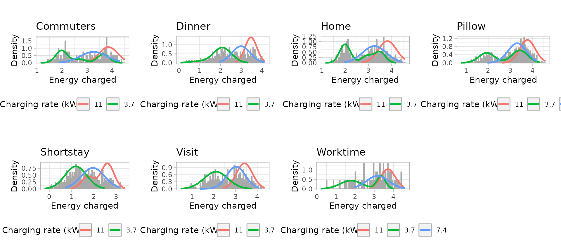
Saturdays models
Connection models: Bi-variate Gaussian Mixture Models
# Build the models
saturday_connection_models <- get_connection_models(
  subsets_clustering = list(
    saturday_city_GMM, saturday_home_GMM
  ),
  clusters_definition = list(
    saturday_city_clusters_profiles, saturday_home_clusters_profiles
  )
)
# Plot the bivariate GMM
saturday_connection_models_plot <- plot_model_clusters(
  subsets_clustering = list(
    saturday_city_GMM, saturday_home_GMM
  ),
  clusters_definition = list(
    saturday_city_clusters_profiles, saturday_home_clusters_profiles
  ),
  profiles_ratios = saturday_connection_models[c("profile", "ratio")],
  log = TRUE
)
Energy models: Uni-variate Gaussian Mixture Models
# Build the models
saturday_energy_models <- sessions_energy_models %>%
  filter(Timecycle == 'Saturday') %>%
  get_energy_models(
    log = TRUE,
    by_power = TRUE
  )
# Plot the univariate GMM
saturday_energy_models_plots <- plot_energy_models(saturday_energy_models)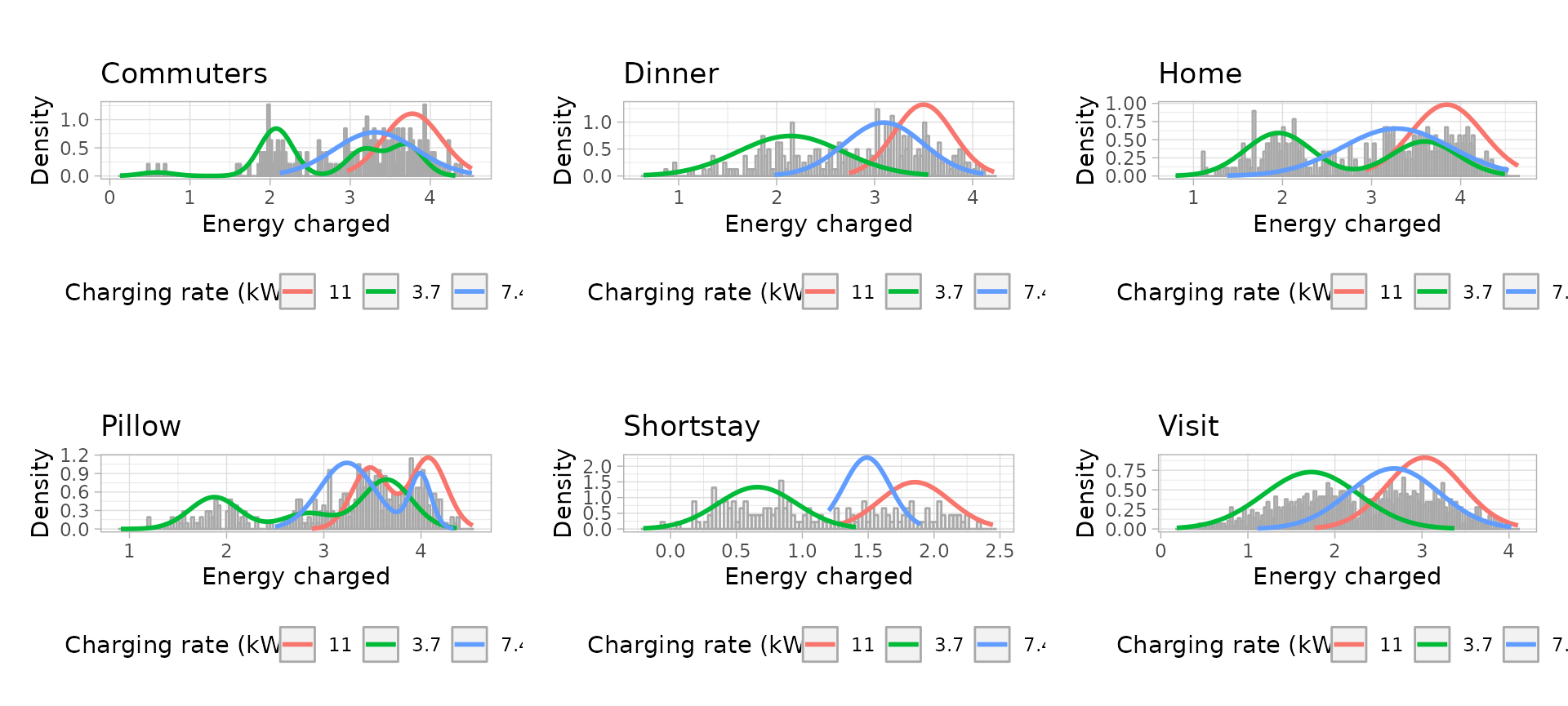
Sundays models
Connection models: Bi-variate Gaussian Mixture Models
# Build the models
sunday_connection_models <- get_connection_models(
  subsets_clustering = list(
    sunday_city_GMM, sunday_home_GMM
  ),
  clusters_definition = list(
    sunday_city_clusters_profiles, sunday_home_clusters_profiles
  )
)
# Plot the bivariate GMM
sunday_connection_models_plot <- plot_model_clusters(
  subsets_clustering = list(
    sunday_city_GMM, sunday_home_GMM
  ),
  clusters_definition = list(
    sunday_city_clusters_profiles, sunday_home_clusters_profiles
  ),
  profiles_ratios = sunday_connection_models[c("profile", "ratio")],
  log = TRUE
)
Energy models: Uni-variate Gaussian Mixture Models
# Build the models
sunday_energy_models <- sessions_energy_models %>%
  filter(Timecycle == 'Sunday') %>%
  get_energy_models(
    log = TRUE,
    by_power = TRUE
  )
# Plot the univariate GMM
sunday_energy_models_plots <- plot_energy_models(sunday_energy_models)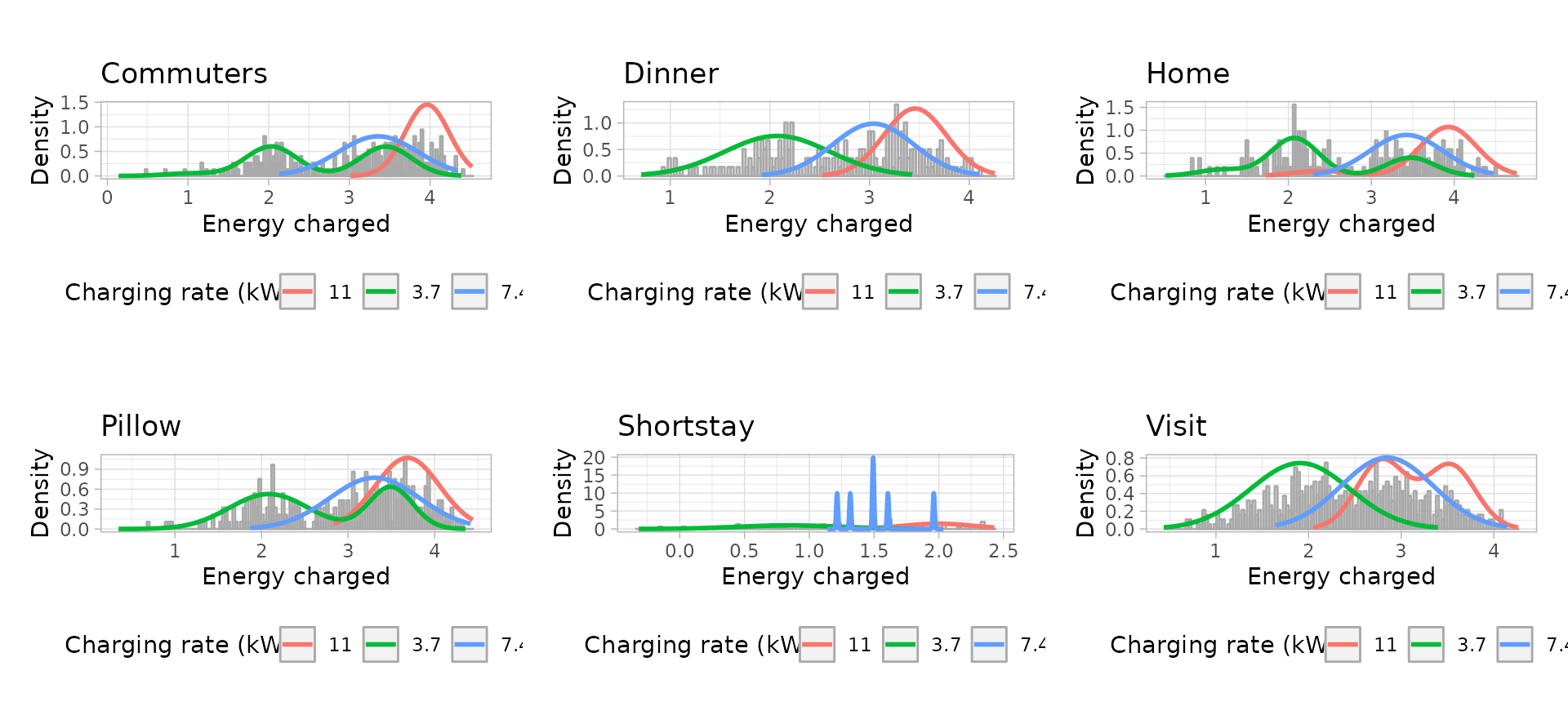
Save the EV model
The package evprof proposes a standard format for the
EV model with the function get_ev_model(). This function
returns an object of class evmodel, which can be used then
as input of evsim package to simulate new sessions. The
function requires the following variables:
-
names: Character vector with the names of the time cycle -
months_lst: List of numeric vectors, each observation containing the months of validity of each time cycle -
wdays_lst: List of numeric vectors, each observation containing the weekdays of validity (week start = 1) of each time cycle -
connection_GMM: List of the connection models returned by functionget_connection_models() -
energy_GMMList of the connection models returned by functionget_energy_models() -
connection_log: logicalTRUEsince we have built the connection models in a logarithmic scale -
energy_log: logicalTRUEsince we have built the energy models in a logarithmic scale -
tzone: In our case the sessions are inEurope/Amsterdamtime-zone
ev_model <- get_ev_model(
  names = c('Workday', 'Friday', 'Saturday', 'Sunday'),
  months_lst = list(1:12),
  wdays_lst = list(1:4, 5, 6, 7),
  connection_GMM = list(
    workday_connection_models, friday_connection_models,
    saturday_connection_models, sunday_connection_models
  ),
  energy_GMM = list(
    workday_energy_models, friday_energy_models,
    saturday_energy_models, sunday_energy_models
  ),
  connection_log = T,
  energy_log = T,
  data_tz = "Europe/Amsterdam"
)

ev_model
## EV sessions model of class "evmodel", created on 2025-04-01
## Timezone of the model: Europe/Amsterdam
## The Gaussian Mixture Models of EV user profiles are built in:
## - Connection Models: logarithmic scale
## - Energy Models: logarithmic scale
##
## Model composed by 4 time-cycles:
## 1. Workday:
## Months = 1-12, Week days = 1-4
## User profiles = Dinner, Shortstay, Visit, Worktime, Commuters, Home, Pillow
## 2. Friday:
## Months = 1-12, Week days = 5
## User profiles = Dinner, Shortstay, Visit, Worktime, Commuters, Home, Pillow
## 3. Saturday:
## Months = 1-12, Week days = 6
## User profiles = Dinner, Shortstay, Visit, Commuters, Home, Pillow
## 4. Sunday:
## Months = 1-12, Week days = 7
## User profiles = Dinner, Shortstay, Visit, Commuters, Home, PillowThen we can save the object to a JSON file with:
save_ev_model(ev_model, file = "arnhem_data/evmodel_arnhem.json")Compare BAU and simulated demand
To simulate new sessions with our models we will make use of package {evsim}. We need the following data:
- Number of sessions of each model
- User profiles proportions for each model
- Charging powers proportions
We will compare the current demand with the demand obtained from our
models for a certain period, for example the two first weeks of
September 2019. The time series demand from a sessions data set can also
be obtained with evsim package, using function
evsim::get_demand().
interval_mins <- 15
start_date <- dmy(01022020) %>% as_datetime(tz = getOption('evprof.tzone')) %>% floor_date('day')
end_date <- dmy(29022020) %>% as_datetime(tz = getOption('evprof.tzone')) %>% floor_date('day')
dttm_seq <- seq.POSIXt(from = start_date, to = end_date, by = paste(interval_mins, 'min'))

sessions_demand <- sessions_profiles %>%
  filter(between(ConnectionStartDateTime, start_date, end_date))

demand <- sessions_demand %>%
  get_demand(dttm_seq = dttm_seq)
We can plot the time-series demand with function
evsim::plot_ts:
To simulate an equivalent type of sessions we have to find the following parameters:
-
EV model: We have probably stored the EV model in a
JSON file so we can read it with function
read_ev_model:
ev_model <- read_ev_model(file = "arnhem_data/evmodel_arnhem.json")-
Charging rates distribution: We can get the current
charging power distribution with function
get_charging_rates_distribution():
charging_rates <- get_charging_rates_distribution(sessions_demand) %>%
  select(power, ratio)

print(charging_rates)
## # A tibble: 7,027 × 2
## power ratio
## <dbl> <dbl>
## 1 0.260 0.000142
## 2 0.340 0.000142
## 3 0.533 0.000142
## 4 0.6 0.000142
## 5 0.68 0.000142
## 6 0.682 0.000142
## 7 0.976 0.000142
## 8 1.02 0.000142
## 9 1.07 0.000142
## 10 1.07 0.000142
## # ℹ 7,017 more rows- Number of sessions per day: The daily number of sessions for each model
n_sessions <- sessions_demand %>%
  group_by(Timecycle) %>%
  summarise(n = n()) %>%
  # Divided by the monthly days of each time-cycle
  mutate(n_day = round(n/c(16, 4, 4, 4))) %>%
  select(time_cycle = Timecycle, n_sessions = n_day)

print(n_sessions)
## # A tibble: 4 × 2
## time_cycle n_sessions
## <fct> <dbl>
## 1 Workday 262
## 2 Friday 261
## 3 Saturday 248
## 4 Sunday 203- Profiles distribution: The user profiles proportion for each model
profiles_ratios <- sessions_demand %>%
  group_by(Timecycle, Profile) %>%
  summarise(n = n()) %>%
  mutate(ratio = n/sum(n)) %>%
  select(time_cycle = Timecycle, profile = Profile, ratio) %>%
  ungroup()

head(profiles_ratios, 10)
## # A tibble: 10 × 3
## time_cycle profile ratio
## <fct> <chr> <dbl>
## 1 Workday Commuters 0.198
## 2 Workday Dinner 0.0886
## 3 Workday Home 0.0829
## 4 Workday Pillow 0.212
## 5 Workday Shortstay 0.152
## 6 Workday Visit 0.204
## 7 Workday Worktime 0.0626
## 8 Friday Commuters 0.0662
## 9 Friday Dinner 0.126
## 10 Friday Home 0.154Finally, the function simulate_sessions() requires the
dates of the simulated sessions and the
interval_mins as the time resolution (in minutes).
Moreover, parameters connection_log and
energy_log must be TRUE if the models have
been built in a logarithmic scale.
With all these parameters in hand we can simulate new sessions:
set.seed(1)
sessions_estimated <- evsim::simulate_sessions(
  evmodel = ev_model,
  sessions_day = n_sessions,
  user_profiles = profiles_ratios,
  charging_powers = charging_rates,
  dates = unique(date(dttm_seq)),
  resolution = interval_mins
)
## # A tibble: 6 × 11
## Session Timecycle Profile ConnectionStartDateTime ConnectionEndDateTime
## <chr> <chr> <chr> <dttm> <dttm>
## 1 S1 Saturday Visit 2020-02-01 08:45:00 2020-02-01 10:45:00
## 2 S2 Saturday Visit 2020-02-01 09:15:00 2020-02-01 10:46:00
## 3 S3 Saturday Visit 2020-02-01 09:15:00 2020-02-01 10:53:00
## 4 S4 Saturday Shortstay 2020-02-01 09:30:00 2020-02-01 10:16:00
## 5 S5 Saturday Visit 2020-02-01 09:30:00 2020-02-01 11:16:00
## 6 S6 Saturday Visit 2020-02-01 09:45:00 2020-02-01 11:48:00
## # ℹ 6 more variables: ChargingStartDateTime <dttm>, ChargingEndDateTime <dttm>,
## # Power <dbl>, Energy <dbl>, ConnectionHours <dbl>, ChargingHours <dbl>Finally, we can calculate the estimated demand and compare it with the real demand:
estimated_demand <- sessions_estimated %>%
  get_demand(dttm_seq = dttm_seq)

comparison_demand <- tibble(
  datetime = dttm_seq,
  demand_real = rowSums(demand[-1]),
  demand_estimated = rowSums(estimated_demand[-1])
)
comparison_demand %>%
  plot_ts(ylab = 'kW') %>%
  dygraphs::dySeries(
    name = 'demand_real', label = 'Real demand', color = 'black',
    strokePattern = 'dashed', strokeWidth = 2
  ) %>%
  dygraphs::dySeries(
    name = 'demand_estimated', label = 'Estimated demand', color = 'navy',
    fillGraph = T
  )
It is obvious that the two demand curves don’t match perfectly because we are not doing a forecasting model but a simulation model, without inputs that predetermine a particular output. What we can compare is the day times where the demand peaks or valleys occur, and this is a positive comparison for our models, which coincide almost perfectly with the real demand. Moreover, the peak values are in general in concordance with the real peaks.