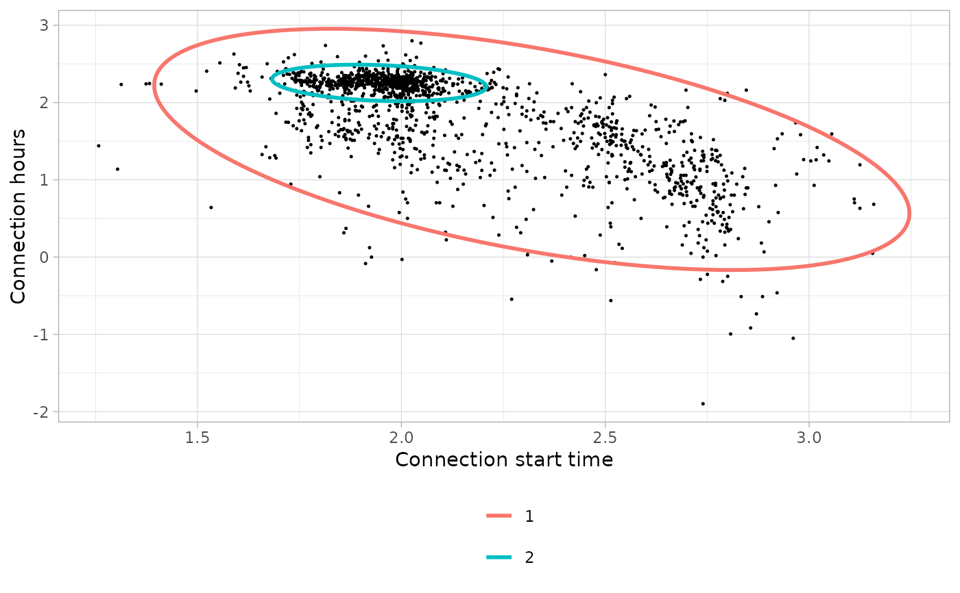
Plot Bivariate Gaussian Mixture Models

Usage

plot_bivarGMM(
  sessions,
  models,
  profiles_names = seq(1, nrow(models)),
  points_size = 0.25,
  lines_size = 1,
  legend_nrow = 2,
  log = FALSE,
  start = getOption("evprof.start.hour")
)

Arguments

sessions: tibble, sessions data set in evprof standard format.
models: tibble, parameters of the clusters' GMM models obtained with function cluster_sessions (object models of the returned list)
profiles_names: names of profiles
points_size: size of scatter points in the plot
lines_size: size of lines in the plot
legend_nrow: number of rows in legend
log: logical, whether to transform ConnectionStartDateTime and ConnectionHours variables to natural logarithmic scale (base = exp(1)).
start: integer, start hour in the x axis of the plot.

Value

ggplot2 plot

Examples

library(dplyr)

# Select working day sessions (`Timecycle == 1`) that
# disconnect the same day (`Disconnection == 1`)
sessions_day <- california_ev_sessions %>%
  divide_by_timecycle(
    months_cycles = list(1:12), # Not differentiation between months
    wdays_cycles = list(1:5, 6:7) # Differentiation between workdays/weekends
  ) %>%
  divide_by_disconnection(
    division_hour = 10, start = 3
  ) %>%
  filter(
    Disconnection == 1, Timecycle == 1
  ) %>%
  sample_frac(0.05)
#> The considered time-cycles are:
#> 
#> 
#> |Timecycle |months |wdays |
#> |:---------|:------|:-----|
#> |1         |1-12   |1-5   |
#> |2         |1-12   |6-7   |
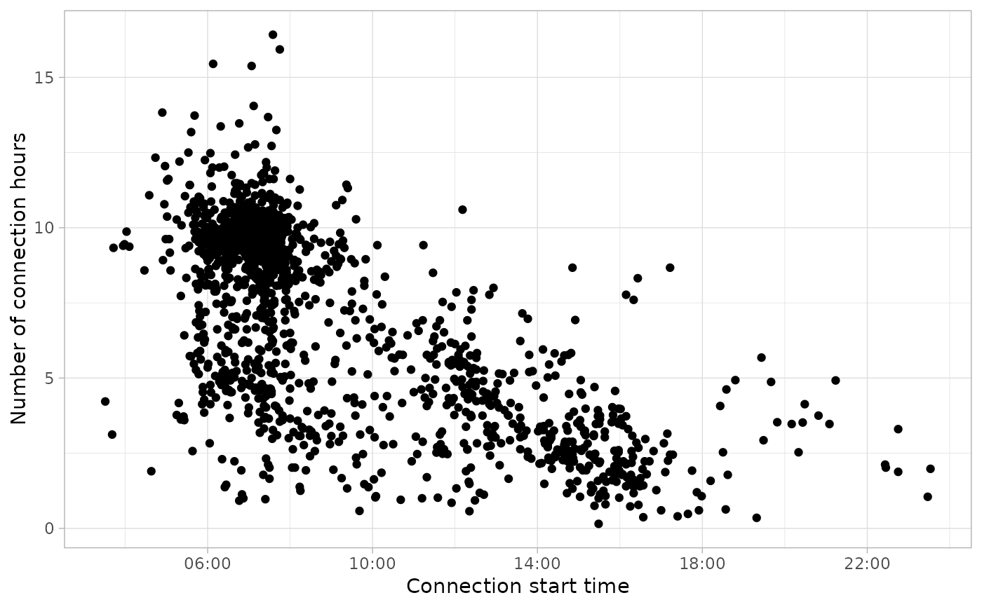
plot_points(sessions_day, start = 3)


# Identify two clusters
sessions_clusters <- cluster_sessions(
  sessions_day, k=2, seed = 1234, log = TRUE
)

# Plot the clusters found
plot_bivarGMM(
  sessions = sessions_clusters$sessions,
  models = sessions_clusters$models,
  log = TRUE, start = 3
)