California case study • evprof

Data exploratory analysis

This case study is based on the open-access data from the California Technological Institute (Caltech) through the ACN Portal initiative. You can download the ACN data set, a collection of EV charging sessions collected at Caltech and NASA’s Jet Propulsion Laboratory (JPL),from the ACN-Data website. For more information visit the ACN documentation.

This data set has been transformed to the standard data format defined by evprof and provided together with the package:

sessions <- evprof::california_ev_sessions

## # A tibble: 30,114 × 12
##    Session ConnectionStartDateTime ConnectionEndDateTime ChargingStartDateTime
##    <chr>   <dttm>                  <dttm>                <dttm>               
##  1 S1      2018-10-08 06:25:00     2018-10-08 17:06:00   2018-10-08 06:25:00  
##  2 S2      2018-10-08 06:35:00     2018-10-08 17:44:00   2018-10-08 06:35:00  
##  3 S3      2018-10-08 06:59:00     2018-10-08 17:28:00   2018-10-08 06:59:00  
##  4 S4      2018-10-08 07:07:00     2018-10-08 17:13:00   2018-10-08 07:07:00  
##  5 S5      2018-10-08 07:07:00     2018-10-08 17:22:00   2018-10-08 07:07:00  
##  6 S6      2018-10-08 07:20:00     2018-10-08 17:37:00   2018-10-08 07:20:00  
##  7 S7      2018-10-08 07:20:00     2018-10-08 17:51:00   2018-10-08 07:20:00  
##  8 S8      2018-10-08 07:27:00     2018-10-08 18:02:00   2018-10-08 07:27:00  
##  9 S9      2018-10-08 07:34:00     2018-10-08 17:20:00   2018-10-08 07:34:00  
## 10 S10     2018-10-08 07:36:00     2018-10-08 17:09:00   2018-10-08 07:36:00  
## # ℹ 30,104 more rows
## # ℹ 8 more variables: ChargingEndDateTime <dttm>, Power <dbl>, Energy <dbl>,
## #   ConnectionHours <dbl>, ChargingHours <dbl>, FlexibilityHours <dbl>,
## #   ChargingStation <chr>, UserID <chr>

For this use case we have to configure the evprof global variable (connections start time) with the following values:

options(
  evprof.start.hour = 3
)

Data set visualization

The ACN charging sessions open data set contains 30114 sessions, from 2018-10-08 06:25:00 to 2021-09-13 22:44:00.

plot_points(sessions, size = 0.5)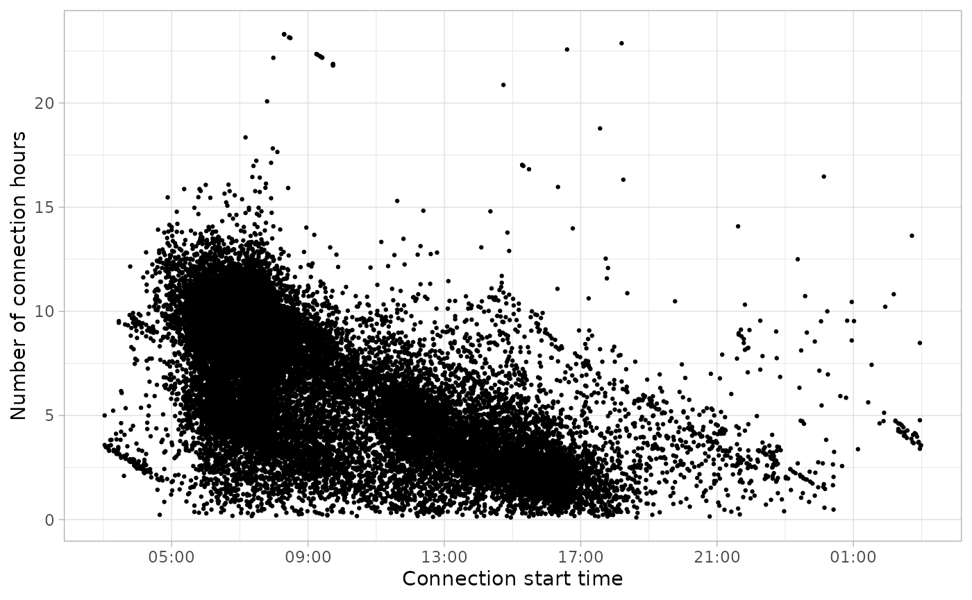

Statistic analysis

The average values of the most important features in our charging sessions data set are:

summarise_sessions(sessions, mean) %>% 
  knitr::kable(digits = 2)

Power	Energy	ConnectionHours	ChargingHours	FlexibilityHours
3.72	14.68	6.89	4.06	2.83

plot_histogram_grid(sessions)

Data preprocessing

Divide the data

Division by Disconnection day

plot_points(sessions, size = 0.25) %>% 
  plot_division_lines(n_lines = 1, division_hour = 6)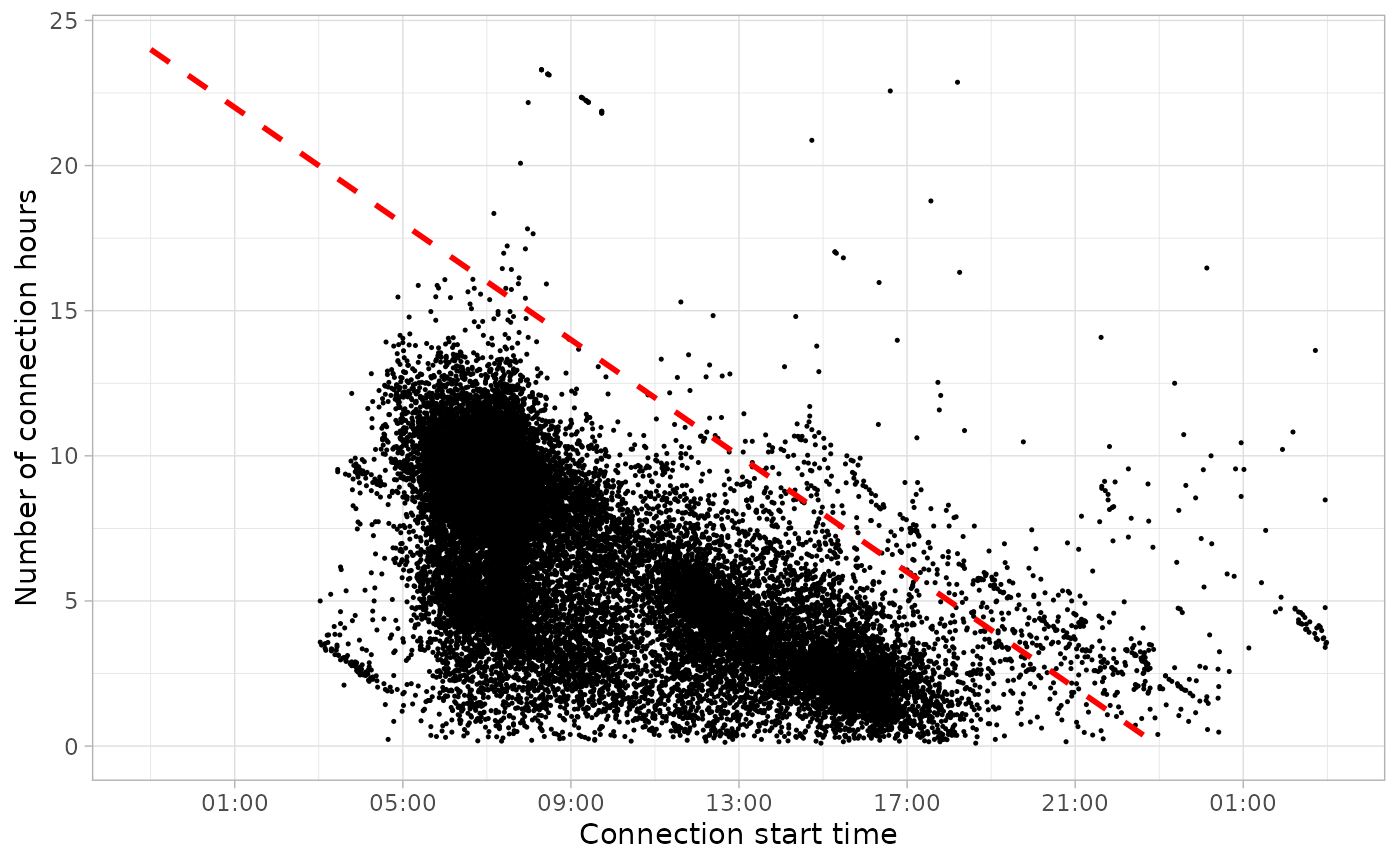

sessions_divisions <- sessions %>% 
  divide_by_disconnection(division_hour = 6) %>% 
  drop_na(Disconnection)

Disconnection day	Number of sessions	Percentage of sessions (%)
1	29474	97.87
2	640	2.13

Time-cycle division

Sessions distribution by day of the week:

plot_density_2D(sessions_divisions, bins = 20, by = 'wday')

Sessions distribution by month:

plot_density_2D(sessions_divisions, bins = 20, by = 'month')

sessions_divisions <- sessions_divisions %>% 
  divide_by_timecycle(months_cycles = list(1:12), wdays_cycles = list(1:5, 6:7))

Time-cycle	Number of sessions	Percentage of sessions (%)
1	29367	97.52
2	747	2.48

Divided data set

Since the sessions disconnecting the day after the connection are not relevant (<2%) we will filter only sessions with Disconnection == "1". Then we change the Timecycle values from 1 and 2 to Workday and Weekend, respectively.

sessions_divided <- sessions_divisions %>% 
  filter(Disconnection == "1") %>%
  mutate(
    Timecycle = plyr::mapvalues(Timecycle, c("1", "2"), c("Workday", "Weekend")),
    Timecycle = factor(Timecycle, levels = c("Workday", "Weekend"))
  ) %>% 
  select(-Disconnection)

head(sessions_divided)

Data cleaning

Let’s see if we have outliers for working days:

sessions_divided %>% 
  filter(Timecycle == "Workday") %>% 
  plot_points(log = T, size = 0.5)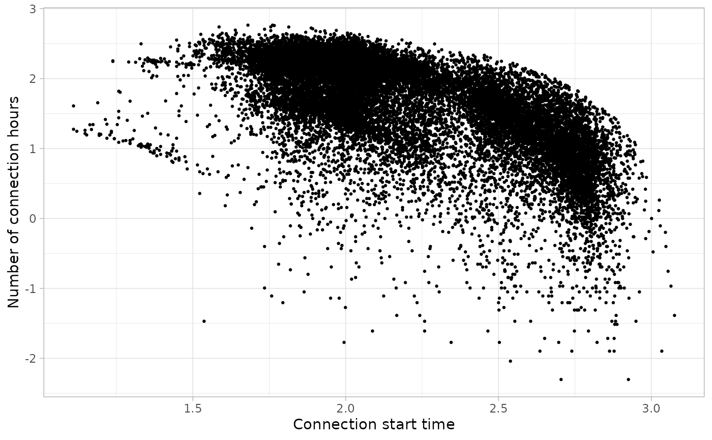

We will cut sessions that start before 1.5 in the logarithmic scale:

sessions_divided %>% 
  filter(Timecycle == "Workday") %>% 
  cut_sessions(connection_start_min = 1.5, connection_hours_min = -1, log = T) %>% 
  plot_points(log = T, size = 0.5)

From this point, it is necessary to iterate over different parameters in detect_outliers function to detect the visible outliers through function plot_outliers. In this case we were happy with MinPts = 50 and noise_th = 2.5.

sessions_workday_noise <- sessions_divided %>% 
  filter(Timecycle == "Workday") %>%
  cut_sessions(connection_start_min = 1.5, connection_hours_min = -1.5, log = T) %>% 
  detect_outliers(noise_th = 2, log = T, MinPts = 100)

sessions_workday_noise %>%
  plot_outliers(log = T, size = 0.5)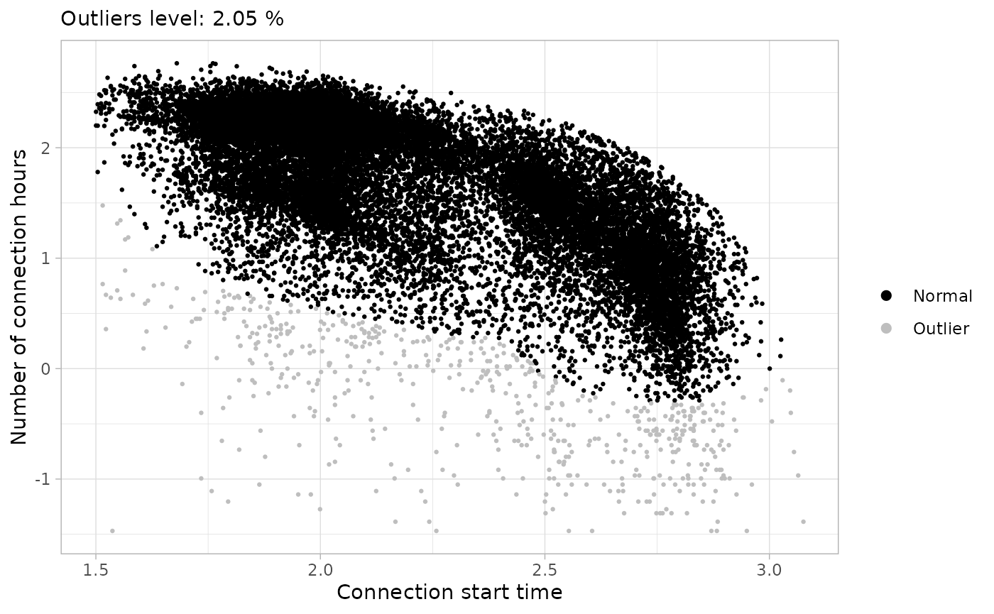

sessions_workday <- sessions_workday_noise %>% 
  drop_outliers()

Let’s repeat the same process for weekends:

sessions_divided %>% 
  filter(Timecycle == "Weekend") %>% 
  plot_points(log = T, size = 0.5)

We will also cut sessions that start before 1.5 in the logarithmic scale., but in this case we consider not necessary to detect outliers with dbscan.

sessions_divided %>% 
  filter(Timecycle == "Weekend") %>% 
  cut_sessions(connection_start_min = 1.5, connection_hours_min = 0, log = TRUE) %>% 
  plot_points(size = 0.5, log = T)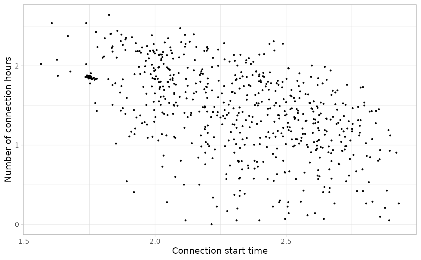

sessions_weekend <- sessions_divided %>% 
  filter(Timecycle == "Weekend") %>% 
  cut_sessions(connection_start_min = 1.8, connection_hours_min = 0, log = TRUE)

The 3D density plot of Workday sessions in logarithmic scale:

plot_density_3D(sessions_workday, log = T)

The 3D density plot of Weekend sessions in logarithmic scale:

plot_density_3D(sessions_weekend, log = T)

Clustering process

Parameters selection

After generating a BIC plot for each one of the 8 sub-sets, the selected number of clusters are:

Sessions workday: k = 6
Sessions weekend: k = 2

Then, each data sub-set has been clustered 6 times and the optimal seeds for each sub-set have resulted as follows:

Sessions workday: seed = 823
Sessions weekend: seed = 484

Clustering

workday_GMM <- cluster_sessions(sessions_workday, k = 6, seed = 823, log = T)
weekend_GMM <- cluster_sessions(sessions_weekend, k = 2, seed = 484, log = T)

bivarGMM_plots <- purrr::map2(
  list(workday_GMM$sessions, weekend_GMM$sessions),
  list(workday_GMM$models, weekend_GMM$models),
  ~ plot_bivarGMM(
    .x, .y, profiles_names = paste0(.y$cluster, " (", round(.y$ratio*100), "%)"), log = T, legend_nrow = 1
  )
)

Profiling

Workday sessions

For workdays’ sessions we differentiate between full-time Workers and Visitors that can connect during the morning, the afternoon or the evening. Basically, the Visit user profile has been assigned to the other clusters that are not connecting during the usual working time.

# Define clusters
workday_clusters_profiles <- define_clusters(
  models = workday_GMM$models,
  interpretations = c(
    "Full-day workers",
    "Full-day or morning visitors",
    "Evening visits",
    "Full-day workers",
    "Full-day workers",
    "Afternoon visits"
  ),
  profile_names = c(
    "Worktime",
    "Visit",
    "Visit",
    "Worktime",
    "Worktime",
    "Visit"
  ),
  log = T
)

workday_clusters_profiles %>% 
  knitr::kable(digits = 2, col.names = c(
    "Cluster", "Controid Start time", "Centroid Connection hours", "Interpretation", "Profile"
  ))

Cluster	Controid Start time	Centroid Connection hours	Interpretation	Profile
1	07:19	9.75	Full-day workers	Worktime
2	12:13	4.73	Full-day or morning visitors	Visit
3	07:26	4.66	Evening visits	Visit
4	07:19	8.90	Full-day workers	Worktime
5	06:33	9.64	Full-day workers	Worktime
6	15:19	2.45	Afternoon visits	Visit

Weekend sessions

In this case we consider that all clusters belong to a Visitor behaviour.

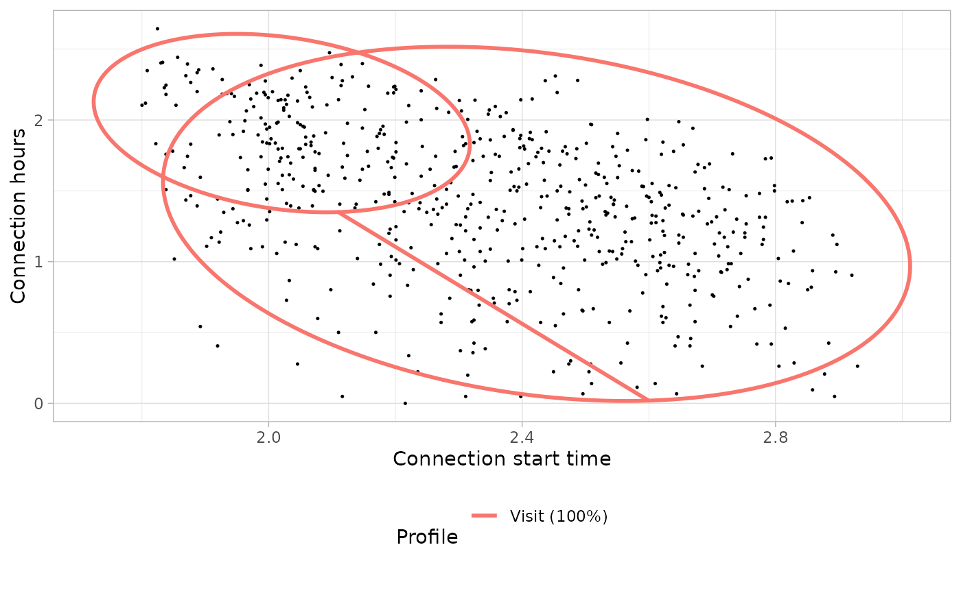
bivarGMM_plots[[2]]

# Define clusters
weekend_clusters_profiles <- define_clusters(
  models = weekend_GMM$models,
  interpretations = c(
    "Morning visitors",
    "Afternoon visits"
  ),
  profile_names = c(
    "Visit",
    "Visit"
  ),
  log = T
)

weekend_clusters_profiles %>% 
  knitr::kable(digits = 2, col.names = c(
    "Cluster", "Controid Start time", "Centroid Connection hours", "Interpretation", "Profile"
  ))

Cluster	Controid Start time	Centroid Connection hours	Interpretation	Profile
1	07:33	7.23	Morning visitors	Visit
2	11:17	3.55	Afternoon visits	Visit

Sessions classification into user profiles

# Join the classification of each subset
sessions_profiles <- set_profiles(
  sessions_clustered = list(workday_GMM$sessions, weekend_GMM$sessions),
  clusters_definition = list(workday_clusters_profiles, weekend_clusters_profiles)
)

head(sessions_profiles)

## # A tibble: 6 × 15
##   Profile  Session ConnectionStartDateTime ConnectionEndDateTime
##   <chr>    <chr>   <dttm>                  <dttm>               
## 1 Worktime S1      2018-10-08 06:25:00     2018-10-08 17:06:00  
## 2 Worktime S2      2018-10-08 06:35:00     2018-10-08 17:44:00  
## 3 Worktime S3      2018-10-08 06:59:00     2018-10-08 17:28:00  
## 4 Worktime S4      2018-10-08 07:07:00     2018-10-08 17:13:00  
## 5 Worktime S5      2018-10-08 07:07:00     2018-10-08 17:22:00  
## 6 Worktime S6      2018-10-08 07:20:00     2018-10-08 17:37:00  
## # ℹ 11 more variables: ChargingStartDateTime <dttm>,
## #   ChargingEndDateTime <dttm>, Power <dbl>, Energy <dbl>,
## #   ConnectionHours <dbl>, ChargingHours <dbl>, FlexibilityHours <dbl>,
## #   ChargingStation <chr>, UserID <chr>, Timecycle <fct>, Cluster <chr>

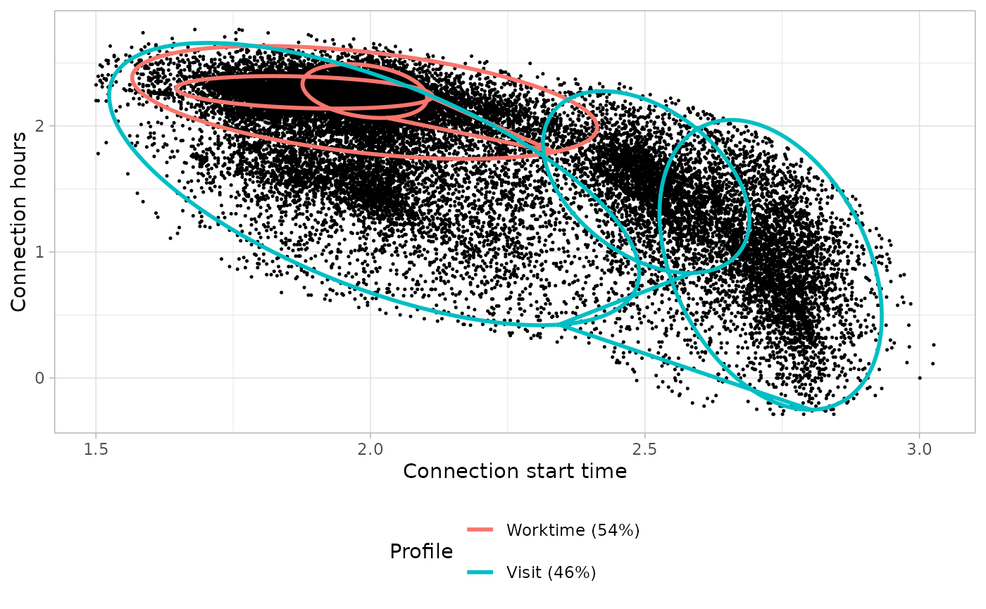
classification_profiles_plot <- plot_points(sessions_profiles, start = 3, log = FALSE, aes(color = Profile), size = 0.3) + 
  facet_wrap(~ Timecycle)

classification_profiles_plot

User profiles modeling

Workdays models

Connection models: Bi-variate Gaussian Mixture Models

# Build the models
workday_connection_models <- get_connection_models(list(workday_GMM), list(workday_clusters_profiles))

# Plot the bivariate GMM
workday_connection_models_plot <- plot_model_clusters(
  list(workday_GMM), list(workday_clusters_profiles), 
  workday_connection_models[c("profile", "ratio")]
)

Energy models: Uni-variate Gaussian Mixture Models

# Build the models
workday_energy_models <- sessions_profiles %>% 
  filter(Timecycle == 'Workday') %>% 
  get_energy_models(
    log = TRUE,
    by_power = FALSE
  )

# Plot the univariate GMM
workday_energy_models_plots <- plot_energy_models(workday_energy_models)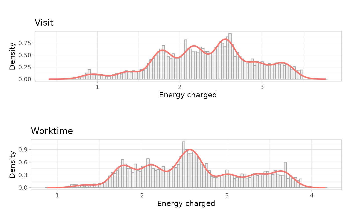

Weekends models

Connection models: Bi-variate Gaussian Mixture Models

# Build the models
weekend_connection_models <- get_connection_models(list(weekend_GMM), list(weekend_clusters_profiles))

# Plot the bivariate GMM
weekend_connection_models_plot <- plot_model_clusters(
  list(weekend_GMM), list(weekend_clusters_profiles), 
  weekend_connection_models[c("profile", "ratio")]
)

Energy models: Uni-variate Gaussian Mixture Models

# Build the models
weekend_energy_models <- sessions_profiles %>% 
  filter(Timecycle == 'Weekend') %>% 
  get_energy_models(
    log = TRUE,
    by_power = FALSE
  )

# Plot the univariate GMM
weekend_energy_models_plot <- plot_energy_models(weekend_energy_models, nrow = 1)

Save the EV models

ev_model <- get_ev_model(
  names = c('Workday', 'Weekend'), 
  months_lst = list(1:12), 
  wdays_lst = list(1:5, 6:7),
  connection_GMM = list(workday_connection_models, weekend_connection_models),
  energy_GMM = list(workday_energy_models, weekend_energy_models),
  connection_log = T,
  energy_log = T,
  data_tz = "America/Los_Angeles"
)

ev_model

## EV sessions model of class "evmodel", created on 2024-03-14 
## Timezone of the model: America/Los_Angeles 
## The Gaussian Mixture Models of EV user profiles are built in:
##   - Connection Models: logarithmic scale
##   - Energy Models: logarithmic scale
## 
## Model composed by 2 time-cycles:
##   1. Workday:
##      Months = 1-12, Week days = 1-2
##      User profiles = Visit, Worktime
##   2. Weekend:
##      Months = 1-12, Week days = 6-7
##      User profiles = Visit

Then we can save the object to a JSON file with:

save_ev_model(ev_model, 'california_data/california_evmodel.json')

Compare BAU and simulated demand

library(dygraphs)
library(lubridate)
library(evsim) # install.packages('evsim')

interval_mins <- 15
start_date <- dmy_hm(090920190000, tz = getOption('evprof.tzone')) # Monday
end_date <-  dmy_hm(290920190000, tz = getOption('evprof.tzone')) + days(1) # Sunday
dttm_seq <- seq.POSIXt(from = start_date, to = end_date, by = paste(interval_mins, 'min'))

sessions_demand <- sessions_profiles %>% 
  filter(between(ConnectionStartDateTime, start_date - days(1), end_date))

demand <- sessions_demand %>% 
  evsim::get_demand(dttm_seq)

We can plot the time-series demand with function evsim::plot_ts:

demand %>% 
  evsim::plot_ts(fillGraph = T)

To simulate an equivalent type of sessions we have to find the following parameters:

Charging rates distribution: We can get the current charging power distribution with function get_charging_rates_distribution():

charging_rates <- get_charging_rates_distribution(sessions_demand) %>% 
  select(power, ratio)

print(charging_rates)

## # A tibble: 2 × 2
##   power ratio
##   <dbl> <dbl>
## 1   3.7 0.798
## 2   7.4 0.202

Number of sessions per day: The daily number of sessions for each time cycle

n_sessions <- sessions_demand %>% 
  group_by(Timecycle) %>% 
  summarise(n = n()) %>% 
  mutate(n_day = round(n/c(20, 8))) %>% # Divided by the monthly days of each time-cycle
  select(time_cycle = Timecycle, n_sessions = n_day)

print(n_sessions)

## # A tibble: 2 × 2
##   time_cycle n_sessions
##   <fct>           <dbl>
## 1 Workday            47
## 2 Weekend             2

Profiles distribution: The user profiles proportion for each time cycle

profiles_ratios <- sessions_demand %>% 
  group_by(Timecycle, Profile) %>% 
  summarise(n = n()) %>% 
  mutate(ratio = n/sum(n)) %>% 
  select(time_cycle = Timecycle, profile = Profile, ratio) %>% 
  ungroup()

print(profiles_ratios)

## # A tibble: 3 × 3
##   time_cycle profile  ratio
##   <fct>      <chr>    <dbl>
## 1 Workday    Visit    0.393
## 2 Workday    Worktime 0.607
## 3 Weekend    Visit    1

Simulate new EV sessions with function simulate_sessions() from package evsim:

sessions_estimated <- simulate_sessions(
  evmodel = ev_model,
  sessions_day = n_sessions,
  user_profiles = profiles_ratios,
  charging_powers = charging_rates, 
  dates = unique(date(dttm_seq)), 
  resolution = interval_mins
)

## # A tibble: 6 × 11
##   Session Timecycle Profile  ConnectionStartDateTime ConnectionEndDateTime
##   <chr>   <chr>     <chr>    <dttm>                  <dttm>               
## 1 S1      Workday   Visit    2019-09-09 05:00:00     2019-09-09 14:20:00  
## 2 S2      Workday   Worktime 2019-09-09 06:00:00     2019-09-09 15:00:00  
## 3 S3      Workday   Worktime 2019-09-09 06:00:00     2019-09-09 16:07:00  
## 4 S4      Workday   Visit    2019-09-09 06:00:00     2019-09-09 13:17:00  
## 5 S5      Workday   Visit    2019-09-09 06:15:00     2019-09-09 15:28:00  
## 6 S6      Workday   Visit    2019-09-09 06:45:00     2019-09-09 11:50:00  
## # ℹ 6 more variables: ChargingStartDateTime <dttm>, ChargingEndDateTime <dttm>,
## #   Power <dbl>, Energy <dbl>, ConnectionHours <dbl>, ChargingHours <dbl>

Finally, we can calculate the estimated demand and compare it with the real demand:

estimated_demand <- sessions_estimated %>% 
  get_demand(dttm_seq)
  
comparison_demand <- tibble(
  datetime = dttm_seq,
  demand_real = rowSums(demand[-1]),
  demand_estimated = rowSums(estimated_demand[-1])
)

comparison_demand %>% 
  plot_ts(ylab = 'kW') %>% 
  dygraphs::dySeries('demand_real', 'Real demand', color = 'black', strokePattern = 'dashed', strokeWidth = 2) %>% 
  dygraphs::dySeries('demand_estimated', 'Estimated demand', color = 'navy', fillGraph = T)

We see that from Monday to Thursday the peak demand from our simulation corresponds quite well with the real peak demand. However, for Fridays it is not so good, so maybe it would be convenient to consider Fridays as a separate time-cycle instead of considering it a normal working day. The demand on weekends is also not really accurate due to the low amount of sessions (~ 3). Obviously, the stochastic simulations work better with large amounts of data since the aggregation makes the random component not so relevant.