Multi-core processing

The time-series calculations done by functions get_demand and get_n_connections can be done by multiple time windows in parallel. At the same time, in computer science, a common practice to reduce computation times is parallel processing when the computer has multiple CPUs (i.e. multi-core processing). In parallel processing, a task is divided into multiple sub-tasks and assigned to multiple cores to make de calculations in parallel. For parallel processing in R we make use of the R base package parallel.

We can discover the number of physical CPUs in our computer with function parallel::detectCores:

n_cores <- parallel::detectCores(logical = FALSE)
print(n_cores)

## [1] 8

We set the parameter logical = FALSE because it is important to know the physical CPUs, not the logical (or virtual/thread) ones seen by the OS. More information about this parameter can be found in parallel::detectCores documentation.

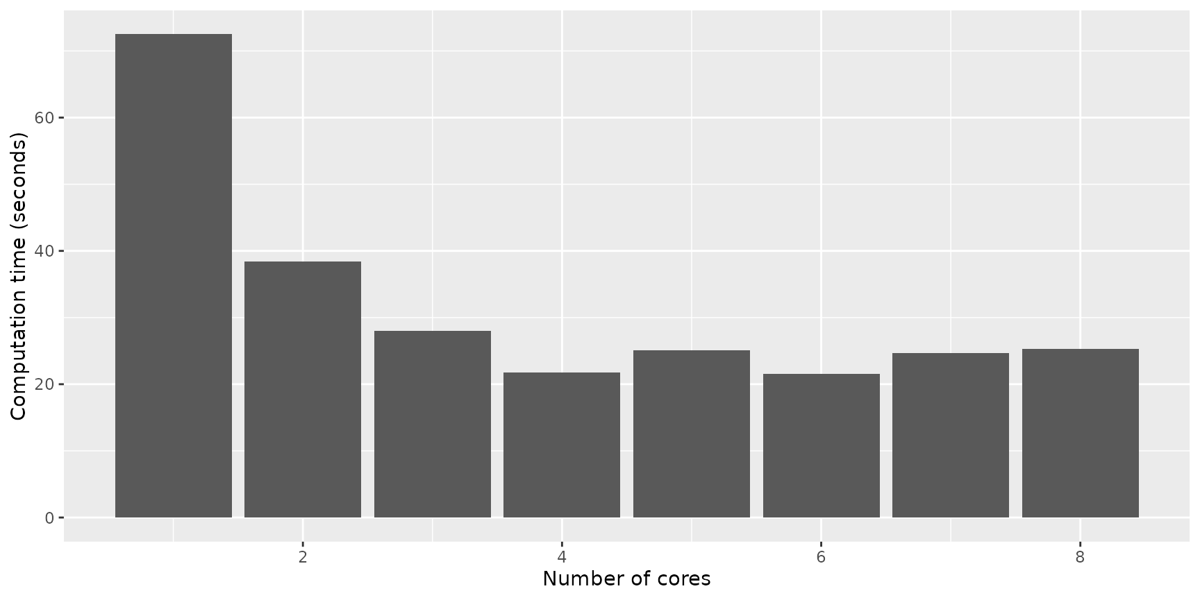
Below, an example of calculating the demand of 10.000 EV charging sessions with different number of cores:

cores_time <- tibble(
  cores = 1:n_cores,
  time = 0
)
for (mcc in cores_time$cores) {
  results <- system.time(
    evsim::california_ev_sessions %>%
       sample_n(10000) %>%
       mutate(Profile = "All") %>%
       get_demand(by = "Profile", resolution = 60, mc.cores = mcc)
  )
  cores_time$time[mcc] <- as.numeric(results[3])
}

And below there’s the plot of the results, were we can see that, for this computer, the optimal number of cores to use is 4:

library(ggplot2)
cores_time %>%
  ggplot(aes(x = cores, y = time)) +
  geom_col() + 
  labs(x = "Number of cores", y = "Computation time (seconds)")